§ 3 Second-order partial differential equations
Classification, standard forms and characteristic equations of first and second order partial differential equations
Consider second order partial differential equations
 (1)
(1)
where a ij ( x ) = a ij ( x 1 , x 2 , … , x n ) is a known function of x 1 , x 2 , … , x n .
[ characteristic equation , characteristic direction , characteristic surface , characteristic plane , characteristic cone ]
Algebraic equations
![]()
is called the characteristic equation of the second-order equation (1) ; here a 1 , a 2 , … , a n are some parameters, and have . If the point x ° =( x 1 ° , x 2 ° , … , x n ° ) satisfy the characteristic equation, that is,![]()
![]()
Then the normal direction l of the plane passing through x ° : ( a 1 , a 2 , … , a n ) is called the characteristic direction of the second-order equation; if a ( n ) dimensional surface, the normal direction of each point is If the direction of the normal line is the characteristic direction, the surface is called the characteristic surface, and the conical surface formed by the envelope of the characteristic plane at one point is called the characteristic surface . Feature cone .![]()
![]()
![]()
[ Classification and standard form of equations with n independent variables ] At point P ( x 1 ° , x 2 ° , … , x n ° ) , according to the quadratic form
![]() ( a i is a parameter )
( a i is a parameter )
The sign of the characteristic root of , the equations can be divided into four categories:
(i) The characteristic roots have the same sign and none of them are zero, so the equation is said to be elliptic at point P.
(ii) None of the eigenvalues are zero, there are n![]() ones with the same sign , and the remaining one has the opposite sign, and the equation is said to be hyperbolic at point P.
ones with the same sign , and the remaining one has the opposite sign, and the equation is said to be hyperbolic at point P.
(iii) None of the eigenvalues are zero, one has the same sign ( n > m > 1) , and the other m have another sign, and the equation is said to be hyper-hyperbolic at point P.![]()
(iv) At least one of the characteristic roots is zero, and the equation is said to be parabolic at point P.
If the equation of each point in region D is elliptic, hyperbolic or parabolic, then the equation in region D is said to be elliptic, hyperbolic or parabolic, respectively .
A linear transformation of the independent variable at point P converts the equation into standard form:
Oval type:![]()
Hyperbolic:
Hyperbolic type:
Parabolic:
where Φ is the term that does not include the second derivative .
[ Classification and Standard Form of Equation with Two Independent Variables ] The general form of the equation is
![]() (2)
(2)
a 11 , a 12 , a 22 are quadratic continuous differentiable functions of x , y , not zero at the same time .
equation
a 11 d y 2 a ![]() 12 d x d y + a 22 d x 2 =0
12 d x d y + a 22 d x 2 =0
It is called the characteristic equation of equation (2) . The integral curve of the characteristic equation is called the characteristic curve of the second-order equation (2 ) .
In the neighborhood D of a point P ( x 0 , y 0 ) , the equations are classified according to the sign of Δ = a 12 2 - a 11 a 12 :
When Δ > 0 , the equation is hyperbolic;
When Δ = 0 , the equation is parabolic;
When Δ < 0 , the equation is elliptical .
By performing variable substitution in the neighborhood D of point P , the equation can be transformed into a standard form:
(i) Hyperbolic: Because Δ > 0 , there are two families of real characteristic curves , , which are transformed , and the equations are transformed into standard forms![]()
![]()
![]()
![]()
![]()
![]()
or
![]()
(ii) Parabolic : Because Δ = 0 , there is only a family of real characteristic curves , take the quadratic continuous differentiable function , make , transform , , and the equation is transformed into a standard form ![]()
![]()
![]()
![]()
![]()
![]()
(iii) Ellipse: Because Δ <0 , there is no real characteristic curve, let
![]()
Integral for , not zero at the same time, make variable substitution , , the equation is transformed into standard form
![]()
![]()
![]()
![]()
2. The
principle of extreme value , energy integration , and the uniqueness theorem of definite solutions
The extreme value principle of elliptic equations, parabolic equations and the energy conservation principle of hyperbolic equations are one of the most basic properties of the solutions of the corresponding equations, and play an important role in the study of definite solutions .
[ Extremum Principle of Elliptic Equations and Uniqueness Theorem of Solutions ]
1 ° Extreme Principle Let D be the bounded region of the n - dimensional Euclidean space En , S is the boundary of D , consider the elliptic equation in D
where a ij ( x ), b i ( x ), c ( x ), f ( x ) are continuous above, c ( x ) ≤ 0 and quadratic positive definite, that is, there is a constant μ > 0 , for any and any The a i have![]()
![]()
![]()
![]()
Theorem 1 Let u ( x ) be the solution of the elliptic equation in D, which is quadratic continuous differentiable in D , continuous in D , and not constant, such as f ( x ) ≤ 0 (or f ( x ) ≥ 0 ) , then u ( x ) cannot take a non-positive minimum (or a non-negative maximum) at an interior point of D. ![]()
If any point P on the boundary S can be made as a ball, making it tangent to S at point P and completely contained in the area D , then we have
Theorem 2 Let u ( x ) be a quadratic continuously differentiable solution of the elliptic equation in D , and it is not a constant, and let f ( x ) ≤ 0 (or f ( x ) ≥ 0 ) . If u ( x ) takes a non-positive minimum value (or a non-negative maximum value) at a point M on the boundary S , as long as the external normal derivative exists at point M , then ![]()
![]()
![]() ( or )
( or )![]()
2 ° Definite solution problem
(i) The first boundary value problem (Dirichlet problem)
![]() ( S )
( S )
(ii) Second boundary value problem (Neumann problem)
![]() ( S )
( S )
where N is the direction of the outer normal of S.
(iii) Third Boundary Value Problem (Mixed Problem)
![]() ( S )
( S )
a ( ), b ( ), ( ) are continuous on S , N is the direction of the outer normal of S, a ( ) ≥ 0 , b ( ) ≤ 0 , and a 2 ( )+ b 2 ( ) ≠ 0 .
The uniqueness of the 3° solution is assumed that c ( x ) and b ( ) are not equal to zero at the same time. If the solution of the definite solution problem Lu=f , lu= exists, it is unique, and both c ( x ) and b ( ) are is equal to zero, if the solution of the definite solution problem Lu=f , lu= exists, then the solution is unique except for a difference of a constant . ![]()
![]()
[ Extremum principle of parabolic equation and uniqueness theorem of solution ] Set as a
cylinder , and consider the parabolic equation inside the cylinder![]()
![]()
![]()
where a ij ( x , t ), b i ( x , t ), c ( x , t ), f ( x , t ) are continuous and positive definite above .![]()
![]()
![]()
1 ° Strong extremum principle Let u ( x , t ) be the continuous solution of the parabolic equation Lu=f ( x , t ) in D × (0, T ) , and let f ( x ) = 0 , if u ( x , t ) takes the non-negative maximum value at a point ( x 0 , t 0 ) of D × (0, T ] , that is ![]()
![]()
Then for any point P ( x , t ) that satisfies the following conditions , there is u ( x , t ) = m : point P ( x , t ) satisfies t < t 0 , and can be completely in D × (0, T ] A continuous curve within x = x ( t ) is connected to the point ( x 0 , t 0 ) .
For example, on the lateral boundary of Γ : S × [0, T ] ( S is the boundary of D ), any point P can be a sphere, making it tangent to Γ at point P and completely at D × (0, T ) inside, there is![]()
Theorem Let u ( x , t ) be continuous on , and satisfy the parabolic equation Lu=f in D × (0, T ] , and it is not a constant, let f ≤ 0 , if u ( x , t ) is at a point on Γ Take the non-positive minimum value at M , as long as the external normal derivative exists at point M , then
![]()
![]()
![]()
2 ° The Cauchy problem and the mixed problem
The initial condition of the Cauchy problem is
![]()
Mixed problems are called according to the following definite solution conditions.
(i) The first boundary value problem: , ;![]()
![]()
(ii) Linear boundary value problem: , ,![]()
where N is a known function of the direction of the outer normal of Γ , a ≥ 0 , b ≤ 0 , a 2 + b 2 ≠ 0![]()
The uniqueness theorem of 3 ° solutions If the solution of the mixture problem of the parabolic equation Lu = f exists , then it is unique . If there is a bounded solution to the Cauchy problem, then the solution is unique in the class of bounded functions .
[ The uniqueness theorem of energy integral and solution of wave equation ]
The Cauchy Problem and Mixed Problem of the 1 ° Wave Equation Let the wave equation be
The initial condition of the Cauchy problem is
![]()
If the wave equation is considered in the bounded region Q : D × (0, T ] , and the lateral boundary is denoted as Γ , the definite solution condition of the mixed problem is![]()
(i)
The first boundary value problem
(ii)
Second boundary value problem
(iii)
The third boundary value problem
where N is the outer normal direction of Γ , φ ( x ), ψ ( x ) are known functions on D , ( , t ) and ( , t ) ( ∈ Γ , 0 ≤ t ≤ T ) are defined in A known function on Γ , ( , t ) ≠ 0 .
The uniqueness theorem of the 2 ° solution The solution of the mixed problem of the wave equation and the Cauchy problem must be unique if it exists .
The uniqueness theorem can be proved by the following energy integration .
3 ° Energy Integral Integral
It is called the energy integral of the wave equation .
The function u ( x , t ) satisfying the homogeneous wave equation and u | Γ =0 (or ) holds:![]()
The principle of conservation of energy E ( t ) = E (0).
energy inequality ![]()
in the formula
![]()
For functions that satisfy the homogeneous wave equation and , adding an item to the above energy inequality E ( t ) , the above relationship still holds .![]()
![]()
For the Cauchy problem , in the characteristic cone
![]() ( R is a constant greater than zero)
( R is a constant greater than zero)
Consider the solution u of the homogeneous wave equation in![]()
Form the following energy inequality
in the formula
![]()
π t is the intersection of the t= constant hyperplane and the cylinder made for the upper base (the generatrix is parallel to the Ot axis) . ![]()
Three,
three typical equations
1. Wave Equation
Study the wave equation of the form
![]()
where f ( x , y , z , t ) is a known function .
The motion laws of many objects can be described by wave equations . For example, the vibration of strings can be described by one-dimensional wave equations; the vibration of membranes can be described by two-dimensional wave equations; the oscillations of sound waves and electromagnetic waves can be described by three-dimensional wave equations .
[ Solution to the Cauchy Problem of Homogeneous Equations ] Let the Cauchy problem of the homogeneous wave equation satisfy the following initial conditions
:
![]()
Assuming that the third time is continuously differentiable and the second time is continuously differentiable, then the expressions for solving u are respectively:![]()
![]()
1 ° three-dimensional (Kirchhoff formula)
where S at represents the spherical surface: , d S represents the area element of the spherical surface .![]()
2 ° two-dimensional (Poisson formula)
where K at represents a circle: .
![]()
3 ° one-dimensional (D'Alembert formula)
![]()
A low-dimensional solution can be derived from a high-dimensional solution by means of dimensionality reduction .
[ Solution to the Cauchy problem of the inhomogeneous equation ] The solution of the Cauchy problem of the inhomogeneous wave equation is equal to the solution of the Cauchy problem of the homogeneous equation above adding a term called delayed potential .
![]()
1 ° 3D
In the formula, the integral area is a sphere with ( x, y, z ) as the center and at as the radius ,
![]()
2 ° 2D
in the formula .
![]()
One-dimensional
![]()
[ Physical meaning of the solution ] The expression of the solution of the wave equation has a clear physical meaning
.
The propagation of a 1 ° wave takes string vibration as an example . In D'Alembert's formula, the solution in the form of ( x-at ) describes that the string vibration propagates to the right at a constant velocity a , and ( x - at ) is called a right-propagating wave, ( x + at ) is the left propagating wave, and a is the wave speed .
Two characteristic lines x = c 1 , x + at=c 2 intersect the x - axis at x 1 , x 2 through the point P ( x, t ) in the 2 ° dependent interval , then the interval [ x 1 , x 2 ] is called a point The dependence interval of P can be seen from D'Alembert's formula that the value at point P is only related to the initial conditions on [ x 1 , x 2 ] , and has nothing to do with the values outside the interval ( x ) , ( x ) .
![]()
3 ° Determine the area through two points x 1 and x 2 ( x 1 < x 2 ) on the x -axis to make characteristic lines respectively
x=x 1 + at , x=x 2![]()
Then the triangular area x 1 + at ≤ x ≤ x 2 ( t >0)
![]()
Called the decision region of [ x1 , x2 ] ( Fig . 14.4( a )) , the value of the solution in the region is completely determined by the initial conditions on [ x1 , x2 ] . Arbitrarily changing the initial conditions in [ x1 , x2 ] x 2 ] , the solution does not change in this region .
Figure 14.4
4 °The influence area passes through two points on the x -axis to draw a characteristic line respectively ![]()
x=x 1 , x=x 2 + at![]()
Area x 1 - at ≤ x ≤ x 2 ( t >0)
![]()
is the region of influence of [ x 1 , x 2 ] ( Fig. 14.4( b )) . In this region, the value of the solution is affected by the initial conditions on [ x 1 , x 2 ] , while outside this region, the value of the solution is Not affected by the initial conditions on [ x 1 , x 2 ], when the area [ x 1 , x 2 ] is reduced to a point x 0 , the area of influence of the point x 0 is the interval on the x -axis ( Figure 14.4( c ))
x 0 ≤ x ≤ x 0 + at ( t >0)![]()
For the two-dimensional wave equation, the point ( x 0 , y 0 , t 0 ) depends on the region of the circle at t = 0 .
( x - x 0 ) 2 +( y - y 0 ) 2 ≤ a 2 t 0 2
At t= 0 , the determination area of the circle ( x - x 0 ) 2 +( y - y 0 ) 2 ≤ a 2 t 0 2 is the area of the cone with ( x 0 , y 0 , t 0 ) as the vertex ( Fig. 14.5( a )).
( x - x 0 ) 2 +( y - y 0 ) 2 ≤ a 2 ( t - t 0 ) 2 ( t ≤ t 0 )
The area of influence of a point ( x 0 , y 0 , 0) on the initial plane t = 0 is a cone ( Fig. 14.5( b )) .
( x - x 0 ) 2 +( y - y 0 ) 2 ≤ a 2 t 2 ( t> 0)
(1)
The influence area of a certain area on the initial plane t = 0 is the area enclosed by the envelope surface of the cone (1) made by each point on this area .
Figure 14.5
For the three-dimensional wave equation, the point ( x 0 , y 0 , z 0 , t 0 ) depends on the sphere at t = 0
( x - x 0 ) 2 +( y - y 0 ) 2 +( z - z 0 ) 2 = a 2 t 0 2
sphere on initial plane t= 0
( x - x 0 ) 2 +( y - y 0 ) 2 +( z - z 0 ) 2 ≤ a 2 t 0 2
The decision area of is the area of the cone with its base and ( x 0 , y 0 , z 0 , t 0 ) as the vertex
( x - x 0 ) 2 +( y - y 0 ) 2 +( z - z 0 ) 2 ≤ a 2 ( t - t 0 ) 2 ( t ≤ t 0 )
On the initial plane t = 0 , the influence area of the point ( x 0 , y 0 , z 0 , 0) is the cone surface
( x - x 0 ) 2 +( y - y 0 ) 2 +( z - z 0 ) 2 = a 2 t 2
( t> 0)
(2)
The influence area of a certain area on the initial plane is the area enclosed by the envelope surface of the cone (2) made by each point above it .
The following essential differences exist in the propagation of two-dimensional and three-dimensional waves .
The 5 ° Huygens principle affects the three-dimensional wave equation , the point ( x 0 , y 0 , z 0 , 0) has an influence region of
( x - x 0 ) 2 +( y - y 0 ) 2 +( z - z 0 ) 2 ≤ a 2 t 2
( t> 0)
If there is an initial disturbance in a certain bounded region Ω , the area affected by this initial disturbance at time t is all the spheres with the point as the center and at as the radius. When t is large enough, this spherical family has inside and outside The envelope surface, the outer envelope surface is called the front front of the propagating wave, and the inner envelope surface is the back front . The part outside the front front represents the area where the disturbance has not yet reached, and the part inside the back front is the wave that has passed. The area between the front and rear fronts is the part affected by the disturbance. In three dimensions, the wave propagation has clear front and rear fronts, which is called Huygens principle or no rear. effect phenomenon .![]()
The dispersion of the 6 ° wave has on the two-dimensional wave equation , the influence area of the point ( x 0 , y 0 ) is
( x - x 0 ) 2 +( y - y 0 ) 2 ≤ a 2 t 2
If there is an initial disturbance in the bounded region Ω , the wave propagation has only the front front and no rear front, so when the initial disturbance of Ω reaches a certain point, the influence of the disturbance on this point will not disappear, but with It gradually weakens with the increase of time . This phenomenon is called the dispersion of the wave, or the wave has an after-effect phenomenon .
2. Heat conduction equation
The general form of the heat conduction equation is
![]()
where f ( x,t ) is a continuous bounded function .
Heat conduction equations describe physical laws such as heat conduction and molecular diffusion .
The initial condition of the Cauchy problem for the n -dimensional heat conduction equation is
![]()
where is a continuous bounded function, and the expression of the solution of the equation is
3. Laplace equation
To study the equilibrium or stability process of gravitational field, static field, magnetic field and some physical phenomena (such as vibration, heat conduction, diffusion), elliptic equations are usually obtained, and the most typical equation is Laplace equation
Δu = 0
and Poisson equation
Δu = ρ
where ρ is a known function, Δ is the Laplace operator,![]()
[ Poisson integral of solution to Dirichlet problem for circle or sphere ] When the region is a circle or a sphere, it
is convenient to use polar coordinates ( r, ) or spherical coordinates ( r , θ , ) , respectively .
The polar form of Δ u = 0 is
![]()
The spherical coordinate form of Δ u = 0 is
![]()
The Poisson integral of the solution to the Dirichlet problem is
When the 1 ° region is a circle, Δ u= 0,
u | r=a = ( ) , the solution is a Poisson integral
![]()
where ( ) is a known continuous function, ( )= ( +2 ) .
When the 2 ° region is a sphere, Δ u= 0,
u | r=a = ( ) , the solution is a Poisson integral ![]()
where ( ) ![]() is a known continuous function,
is a known continuous function,
![]()
[ Properties of Harmonic Functions ] The continuous solution of the two-dimensional Laplace equation is called a harmonic function
, which has the following important properties:
1 ° Let the function u ( x , y ) be reconciled in a bounded region D bounded by S , and there is a continuous first-order partial derivative on , then ![]()
![]()
where is the external normal derivative .![]()
2 ° Arithmetic Mean Theorem Assuming that the function u ( x,y ) is harmonic inside a circle and continuous on a closed circle, then the value of u ( x,y ) at the center of the circle is equal to the arithmetic mean of its values at the circumference .
3 ° Each harmonic function u ( x , y ) is infinitely differentiable with respect to x, y .
4 ° Hallack's first theorem (uniform convergence theorem) Let { u k ( x,y )}, ( k =1,2 ) be harmonic in the bounded region D , continuous on , if u k ( x,y ) ) converges uniformly on the boundary of D , then it converges uniformly in D , and the limit function is harmonic in D.
![]()
![]()
5 ° Hallack's second theorem (monotonicity theorem) Let the harmonic function sequence { u k ( x,y )}, ( k =1,2, … ) converge at an interior point of D , and for any k ,
u k + 1 ( x,y )≥ u k ( x,y )
Then u k ( x, y ) converges to a harmonic function everywhere in D , and converges uniformly on every bounded closed subregion of D.
6 ° Liuville's Theorem If the function u ( x,y ) is harmonic in the whole plane and not constant, it cannot have upper and lower bounds .
7 ° The theorem of de-singularity Let u ( x,y ) be harmonic and bounded in a neighborhood of point A (except point A ), but not defined at point A , then the function u ( x,y ) can be defined in The value of point A such that u is a harmonic function within the entire neighborhood of point A (including point A ) .
[ Lyapunov closed surface and inner and outer boundary value problem ] Let S be a finite closed surface of En , if the following conditions are satisfied, then S is called a Lyapunov closed surface :
(i) The surface has tangents everywhere .
(ii) There is a constant d> 0 , for each point P on the surface, a sphere with P as the center and d as the radius can be made, so that the part of the surface in this sphere intersects any line parallel to the normal to the point P no more than a little
(iii) The angle γ ( P 1 , P 2 ) between the normals of any two points P 1 and P 2 on the surface satisfies
![]()
where A , δ are constants, 0< δ ≤ 1 , is the distance between points P 1 and P 2 .![]()
(iv) The solid angle of any part σ of the surface viewed from any point P 0 in space is bounded, that is,
| | ≤ k ( k is a constant)
( The solid angle of surface S viewed from point P 0 is
where represents a vector , N P represents the outer normal vector of S at point P , d S P represents the area element of point P. )![]()
![]()
Let D be the bounded region of En, and its boundary S is the Lyapunov closed surface .
Δu = 0
The solution that satisfies the given boundary conditions on S is called an inner boundary value problem; the solution that satisfies Δu = 0 outside D and satisfies the given boundary conditions on S is called an outer boundary value problem .
[ Solution to Dirichlet's problem and Neumann's problem ]
Dirichlet's problem Δ u =0 ,
![]()
Neumann problem Δ u =0 ,
![]()
where M S ∈ S , is a known continuous function on S , and is the external normal derivative .![]()
![]()
The solution to the 1 ° Dirichlet problem can be expressed as an area integral
![]() .
.
where v ( P ) is called areal density, the area fraction u ( M ) is called double-layer potential, r PM is the distance between point M and point P , r PM is a vector , N P is S at point P The outer normal vector of , v ( M ) satisfies the Fredholm integral equation of the second kind ( Chapter 15 § 1) : ![]()
(i) Internal boundary value problem
(ii) Outer value problem
The solution to the 2 ° Neumann problem can be expressed as an area integral
![]()
where ( P ) is called the areal density, the area integral u ( M ) is called the monolayer potential, and ( P ) satisfies the second kind of Fredholm integral equation:
(i) Internal boundary value problem
(ii) Outer value problem
Theorem: Dirichlet's inner and outer boundary value problem and Neumann's outer boundary value problem have unique solutions, and the necessary and sufficient conditions for the existence of solutions to Neumann's inner boundary value problem are:
![]()
[ Poisson equation ] In the region D ,
the Poisson equation Δ u = ρ ( ρ is a known continuous function) has a specific solution:
3D: body position
![]()
2D: Log Potential
![]()
where r PM is the distance between the point M and the change point P.
If a particular solution U ( M ) of the Poisson equation is known , then =u - U satisfies Δ = 0 , so the boundary value problem of the Poisson equation can be transformed into the corresponding boundary value problem of the Laplace equation .
4.
Basic solution and generalized solution
[ Conjugate Differential Operator and Self-Conjugate Differential Operator ] Operator
It is called a second-order linear differential operator, where a ij , b i , c are quadratic continuous differentiable functions of x 1 , x 2 , … , x n . By the formula
The determined operator L * is called the conjugate differential operator of L. If L=L* , then L is called the self-conjugate differential operator .
[ Green formula ]
The Green's formula for the 1 ° operator L is
![]()
where S is the boundary of the region D , N is the outer normal vector of S , and e i is the vector of the axis of x i
(0, … ,0 , ,0, ![]() … ,0),
… ,0),
cos( N , e i ) represents the cosine of the angle between the vector N and e i ,
Green's formula for 2 ° three-dimensional Laplacian
![]()
where is the outer normal derivative .![]()
3 ° operator
![]()
Green's formula
where L* is the conjugate differential operator of L, N is the outer normal vector, i and j are the unit vectors on the x - axis and the y -axis, respectively .
[ Basic solution ]
Fundamental solution of the 1 ° equation Lu=f :
Let M , M 0 be the points in En that satisfy the equation
The solution U ( M, M 0 ) is called the fundamental solution of the equation Lu=f , sometimes also called the fundamental solution of the equation Lu= 0 , where ( MM 0 ) is called the n -dimensional Dirac function ( -function ) .
The basic solution U ( M, M 0 ) satisfies
(i) LU ( M, M 0 )=0 , when M ≠ M 0 ,
(ii) For any sufficiently smooth function f ( M ) ,
![]()
So U ( M, M 0 ) satisfies Lu=f ( M ) .
Therefore, the function U ( M, M 0 ) satisfying the conditions (i) and (ii) is sometimes defined as the basic solution of the equation Lu=f ( M ) .
( a ) Basic solution for Δ u = 0
2D:
![]()
3D:
![]()
n dimension:
where is the distance between point M and M0 .![]()
( b ) The fundamental solution of the multiharmonic equation m u = 0 in n -dimensional space
( c ) Basic solution of heat conduction equation
( d ) Fundamental solution of the wave equation
One-dimensional:
2D:

3D:
2 ° Basic solution to the Cauchy problem
(i) Satisfaction
The solution of is the fundamental solution of the Cauchy problem of the wave equation, which has the form
One-dimensional:
2D:
3D:
![]()
(ii) said to satisfy
The solution of the heat conduction equation is the basic solution of the Cauchy problem, and its form is
In the same way, basic solutions to other definite solutions can be defined .
It can be seen from the definition that the basic solution represents the solution generated by the concentrated quantity (such as point heat source, point charge, etc.), the Green's function and Riemann function introduced in the next paragraph also have this feature, and they are collectively referred to as point source function, or influence function .
[ Generalized solution ] Given a second-order linear equation in region D
where f is continuous on D.
1 ° Let u n ( x ) be a sufficiently smooth (such as second-order continuously differentiable) function sequence on D , when n → ∞, u n ( x ) converges uniformly (or in an appropriate sense) to the function u ( x ) ) , and Lu n also converges consistently (or in an appropriate sense) to f ( x ) , then u ( x ) is called a generalized solution of Lu=f .
2 ° Let the function u ( x ) be continuous in the region D , if for any quadratic continuous differentiable and always equal to zero at the point whose boundary distance from D is less than a certain positive number ( and irrelevant, called the test of D function) has
![]()
Then u ( x ) is called a generalized solution of the equation Lu=f .
Sometimes in order to distinguish the generalized solution, the previously defined solution is called the classical solution, and the classical solution must be the generalized solution . However, because the generalized solution is not necessarily smooth or even non-differentiable, it is not necessarily the classical solution .
For example, when ( x ) , ( x ) is just a continuous function of x, the function
u ( x,t )=( x + t )-( x - t )
is the wave equation
![]()
The generalized solution of , but not the classical solution .
5.
Common solutions of second-order partial differential equations
1. Separation of variables method
It is a commonly used method for solving linear differential equations, especially when the region is a rectangle, a cylinder, or a sphere . The linear combination of , and the solution of the definite solution problem is obtained . The specific solution often boils down to finding the eigenvalues and eigenfunctions of some boundary value problems of ordinary differential equations . The following describes the specific solutions of the separation of variables method for different types of equations .
[ String vibration equation ]
The Mixing Problem of Homogeneous Equations of String Vibration with Fixed Both Ends of 1 °
Let u ( x,t ) = X ( x ) T ( t ) , the specific solution is as follows:
(1) The ordinary differential equation satisfied by X ( x ) and T ( t ) :
(2) Use the product of the solutions of these two ordinary differential equations to express the special solution u n ( x ,t ) of the string vibration equation .
Solving Boundary Value Problems
when
![]()
, there is a non-zero solution
![]()
We call λ n the eigenvalue of the boundary value problem, and X n ( x ) is the eigenfunction . Substituting λ n into the equation of T ( t ) , we get
![]()
In the formula, A n , B n are arbitrary constants, so that the special solution of the string vibration equation can be obtained:
![]()
(3) Add u n ( x , t ) to form a series
![]()
(4) Using the orthogonality of the characteristic functions, determine the coefficients A n , B n .
Expand ( x ) and ( x ) into a Fourier series
in the formula
Using the initial conditions, we can get
![]()
So the mixed problem can be solved in the form of
![]()
If (i) ( x ) has first and second continuous derivatives, the third derivative is continuous piece by piece, and (0) = ( l ) , " (0) = " ( l )=0;(ii) ( x ) Continuously differentiable, the second derivative is continuous piece by piece, (0)= ( l )=0 , then the series on the right-hand side of the formal solution converges uniformly, and the formal solution is the normal solution of the mixed problem .
Physical meaning of the 2 ° solution
![]()
This form of vibration of the string is called a standing wave, and the point
( m = 0,1 n ) is a stationary point, called a node; the point
( m = 0 , 1, 2 n - 1) has the largest amplitude and is called The antinode; called the natural frequency of the string vibration; the frequency of the lowest note emitted by the string is ( τ is the tension, ρ is the linear density of the string) is called the fundamental tone of the string, and other frequencies are integer multiples of it, called Overtones .![]()
![]()
![]()
![]()
![]()
![]()
Mixed Problems of 3 ° Inhomogeneous Equations
Expand u ( x , t ) and f ( x , t ) into a Fourier series:
Then , using the Fourier expansions of ( x ) and ( x ) in 1 ° according to the definite solution conditions, we have
so
![]()
The form is solved as
![]()
If ( x ) has first and second-order continuous derivatives, the third-order derivatives are continuous piece by piece, ( x ) and f ( x,t ) are continuously differentiable, and the second-order derivatives are continuous piece by piece, while
(0) = ( l )= " (0)= " ( l )=0
(0) = ( l )= f (0 ,t )= f ( l,t )=0
Then the series converges uniformly, and the formal solution is the normal solution of the mixture of inhomogeneous equations .
4 ° encounters inhomogeneous boundary conditions
make a transformation
![]()
It can be solved as a homogeneous boundary condition on v ( x,t ) .
[ Heat conduction equation ] The first boundary value problem of the heat conduction equation
Let u ( x,t ) = X ( x ) T ( t ) , we get
X" ( x )+ 2 X ( x )=0
T' ( t )+ a 2 2 T ( t )=0
eigenvalue , the corresponding eigenfunction is , and![]()
![]()
![]()
![]()
make a formal solution
where c n is equal to the Fourier coefficient of ( x ) ie .![]()
When ( x ) has first and second-order continuous derivatives, and the third-order derivatives are continuous piece by piece, (0)= ( l )=0 , then the above series converges uniformly, and the formal solution is a regular solution .
[ Laplace's equation ] Dirichlet's problem for steady temperature distribution in a sphere
- Dirichlet's problem for Laplace's equation .
choose spherical coordinates
Let u ( r, ,![]() ) = v ( r,
) = v ( r,![]() ) ( )
) ( ) ![]() . Substitute into the equation and separate the variables to get
. Substitute into the equation and separate the variables to get![]()
" ( )+ k 2 ( )=0 (1)![]()
![]()
![]() (2)
(2)
Using the periodicity of variables , u ( r, , ) = u ( r,
, + 2 ) , we know that k in equation (1) can only take m ( m = 0,1 ) , then ( ) takes {cos m , sin m } . Then the equation (2 ) is separated into variables , let v = R ( r ) H ( ) , we get![]()
![]()
![]()
![]()
![]()
![]()
![]()
![]()
![]()
![]()
![]() (3)
(3)
![]() (4)
(4)
The solution of equation (4) can be represented by Legendre polynomials. In order to make the solution bounded, λ can only take
λ n 2 = n ( n+ 1) ( n= 0,1,2, … )
The corresponding solution H ( )= P ![]() n ( m ) (cos )
n ( m ) (cos ) ![]() , , P n ( x ) is the Legendre polynomial
, , P n ( x ) is the Legendre polynomial![]()
![]()
Equation (3) can be written as
![]()
This is Euler's equation, and its bounded solution is R ( r ) = c 1 r n . Finally , the special solutions of u are superimposed, and the orthogonality of the boundary conditions and spherical functions is used to obtain
![]()
where P n ( m ) (cos ) ![]() is a general Legendre function .
is a general Legendre function .
If the quadratic is continuously differentiable, then the represented series converges uniformly, and it is the solution of Dirichlet's problem .![]()
![]()
[ Higher-Order Equation ] The lateral vibration equation of the beam is
![]() ( a is a constant)
(1)
( a is a constant)
(1)
The solution condition is
Let y ( x,t )= X ( x ) T ( t ) , then
Equation (2) satisfies the eigenvalue of X" (0) = X" ( l )=0 , the eigenfunction
( n =1,2 ) , the solution of equation (3) is![]()
![]()
![]()
![]()
So the formal solution of equation (1) is
![]()
By y ( x, 0) = x ( l - x ) we get
Finally, the solution of equation (1) is obtained .
2. Riemann method for hyperbolic equations
Consider Laplace's hyperbolic equation
![]()
[ Characteristic line method of ancient sand problem ] The ancient sand problem is
Let a ( x,y ), b ( x,y ), c ( x,y ), f ( x,y ) be continuous functions; continuous differentiable sum , let![]()
![]()
![]()
Then the ancient sand problem can be transformed into the solution of the following integral equations
|
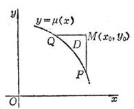
Figure 14.6 |
It can be solved by the successive approximation method, obviously x=x 0 , y=y 0 is the characteristic line of the Laplace hyperbolic equation, so this method is also called the characteristic line method .
[ The Riemann method of the generalized Cauchy problem ] The generalized Cauchy problem is
Let a ( x,y ), b ( x,y ), c ( x,y ), ![]() 1 ( x ) and ( x ) be continuously differentiable functions, and ' ( x ) ≠ 0 , and f ( x,y ) ) and 2 ( x ) are continuous functions .
1 ( x ) and ( x ) be continuously differentiable functions, and ' ( x ) ≠ 0 , and f ( x,y ) ) and 2 ( x ) are continuous functions .![]()
Suppose M ( x 0 , y 0 ) is not a point on y= ( x ) , and draw a characteristic line x=x 0 , y=y 0 through point M and intersect y= ( x ) at P and Q , denote a curved triangle PMQ is D (Fig. 14.6 ), using Green's formula (this section, IV) on D to get
Let v ( x,y ; x 0 , y 0 ) be the solution to the following Gusa problem:
Then the Riemann formula for the solution of the generalized Cauchy problem is
where v ( x, y ; x 0 , y 0 ) is called the Riemann function, and this method is called the Riemann method .
Generally, the characteristic line method can be used to find the Riemann function . But for constant coefficient partial differential equations
![]() ( c is a constant)
( c is a constant)
You can also use the following method to find the Riemann function . Set v = v ( z ) , , then the equation can be transformed into a Bessel equation![]()
![]()
The Riemann function is the zero-order Bessel function that satisfies this Bessel equation and the condition v (0)=1 ,
![]()
The Laplace hyperbolic equation for constant coefficients can be transformed into
![]()
, and its Riemann function is the above formula .
3. Green's method for elliptic equations
Consider elliptic equations in region D
![]()
where a ij , b i , c,f are continuous differentiable functions of x 1 , … , x n , a ij = a ji , the quadratic form is positive definite .![]()
[ Green's function and its properties ] If
the basic solution G ( x , ) of the conjugate equation L*u = 0 of Lu = 0 satisfies on the boundary S of D
G ( x , ) = 0, x ∈ S
Then G ( x , ) is called the Green’s function of the equation Lu= 0 , where x = ( x 1 , … , x n ) , ξ is the parameter point, = ( 1 , … , n ) , that is, G ( x , )= G ( x 1 , … , x n ; 1 , … , n ) .
The Green's function has symmetry properties: let G ( x , ), V ( x , ) be the Green's function of the equation Lu= 0 and its conjugate equation respectively, then the symmetry relationship is established
G ( x , ) = V ( x , )
In particular, if Lu is a self-conjugate differential operator, then we have
G ( x , ) = G ( , x )
[ Solving Boundary Value Problems Using Green's Function ]
1 ° General formula Applying Green's formula (this section, 4) on the region D , and taking v=G ( x , ) , the solution of the Dirichlet problem u | s = of the equation Lu=f is ![]()
![]()
in the formula
![]() ( N is the direction of the outer normal of S )
( N is the direction of the outer normal of S )
2 ° For a sphere (the center of the sphere is O and the radius is a ), the basic solution for u = 0 is , r is the distance between P ( x , y, z ) and the parameter point M ( , , ) , and M is about the sphere. Invert the point M 1 , record r 1 as the distance between M 1 and P , then the Green's function is ![]()
![]()
![]() . The solution to the Dirichlet problem u | s = is
. The solution to the Dirichlet problem u | s = is
where S is a spherical surface . When citing spherical coordinates, the solution is a Poisson integral ( this section, 3, 3).
3 ° on a circle (radius a ), the Green's function for u = 0 is
In the formula, r is the distance between P ( x,y ) and the parameter point M ( , ) , r 1 is the distance between P and M point about the inversion point M 1 of the circle, the solution of the Dirichlet problem on the circle is Poisson Points .
4. Integral transformation method
The integral transformation method is an effective method for solving linear differential equations, especially equations with constant coefficients. Convert the equation into a simple form (the simplest case is an ordinary differential equation, or even an algebraic equation) . Solve the corresponding definite solution problem of this simplified equation and obtain the solution of the original definite solution problem through the inverse integral transformation . The following examples illustrate Fourier transform and Laplace transform methods .
Example 1 The Cauchy Problem of Solving String Vibration Equations by Fourier Transform
The solution takes t as a parameter and takes the Fourier transform of u ( x,t ) about x
F![]()
The original Cauchy problem is transformed into the following definite solution problem
Considering p as a parameter, the solution is
![]()
The solution of the original problem is obtained by the inversion formula of the Fourier transform
Example 2 Using Laplace Transform to Solve the Definite Solution of Heat Conduction Equation
The solution takes x as a parameter and takes the Laplace transform of u ( x,t ) with respect to t
L![]()
The original problem becomes

The general solution is
![]()
The solution is required to be bounded . c 2 must be zero, so ,![]()

The Charaplacian transformation table (Chapter 11) has
![]()
where erfc( y ) is the residual error function .