Chapter 16
Probability Statistics and Stochastic Processes
This chapter briefly introduces the important contents of probability theory, in addition to introducing random events and their probability, random variables and distribution functions, numerical characteristics of random variables, probability generating functions, moment generating functions and characteristic functions, law of large numbers and central limit theorem, etc. In addition to basic concepts , the normal distribution table and the use of probability paper are also introduced. This chapter focuses on describing the commonly used mathematical statistics methods, including samples and their frequency distribution, interval estimation of population parameters, statistical testing, variance analysis, regression analysis, orthogonal experimental design, sampling inspection, quality assessment (process control), etc. Finally, the basic content of stochastic process theory is briefly described, and the more commonly used Markov processes and stationary stochastic processes are highlighted.
§ 1 Probability Theory
1.
Events and Probability
1. Random events and their operational relationships
[ Random event · inevitable event · impossible event ] Under certain conditions, the experimental results that may or may not occur are called random events, or events for short, represented by A , B , C , . . . There are two special cases of random events, namely inevitable events (events that must occur in each trial under certain conditions) and impossible events (events that must not occur in each trial under certain conditions), respectively recorded as Ω and Φ .
[ Operational relationship of events ]
1 ° contains When event B occurs , event A must also occur, then A contains B or B is contained in A , denoted as A B , or B A . ![]()
![]()
2 ° Equivalence If A B and A B , that is, events A and B occur at the same time or do not occur, then A and B are said to be equivalent, denoted as A=B . ![]()
![]()
The 3 ° product represents the simultaneous occurrence of events A and B , called the product of A and B , denoted as A B ( or AB ). ![]()
4 °Sum means the event that event A or event B occurs, called the sum of A and B , and denoted as A B ( or A+B ). ![]()
A 5 ° difference represents an event where event A occurs and event B does not, called the difference between A and B , denoted as A \ B (or A ). ![]()
6 ° Mutual exclusion If events A and B cannot occur at the same time, namely AB , then A and B are said to be mutually exclusive (or mutually incompatible). ![]()
7 ° Opposition If events A and B are mutually exclusive, and either A or B occurs in each trial , that is, A B = and A B = Ω , then B is called the opposite event of A , and denoted as B = . ![]()
![]()
![]()
![]()
8 ° Complete If events A 1 , A 2 , ··· , An occur at least one in each trial, that is , { A 1 , A 2 , ··· , An } is said to constitute a complete set of events . Especially when A 1 , A 2 , ··· , An are mutually exclusive in pairs, that is , A i A j = ( ij , i , j = 1 , 2 , ··· ,
![]()
![]()
![]()
![]()
![]() n ), it is said that { A 1 , A 2 , ... , A n } is a complete set of mutually exclusive events.
n ), it is said that { A 1 , A 2 , ... , A n } is a complete set of mutually exclusive events.
2. Several definitions of probability
[ Frequency and Probability ] Whether or not a random event occurs in an experiment is an accidental phenomenon that cannot be determined in advance, but when repeated experiments are carried out, the statistical regularity of the probability of its occurrence can be found. Specifically, if n repeated trials are carried out under the same conditions , and event A occurs v times, then the frequency of event A in n trials appears stable when n increases infinitely. This statistical regularity shows that the possibility of event A happening is an objective attribute inherent in the event itself and not changed by people's subjective will. The probability of event A occurring is called the probability of event A , denoted as P ( A ) . When the number of trials n is large enough, the frequency of the event can be used to approximate the probability of the event, that is![]()
![]()
[ Classical definition of probability ] Suppose a random experiment (an experiment whose outcome cannot be accurately predicted in advance and can be repeated under the same conditions) has only a finite number of different basic events ω 1 , ω 2 , . . . , ω n (A basic event is also a kind of event, a general event is always composed of several basic events), each basic event is equally possible * , the whole of the basic events is recorded as Ω , and it is called the basic event space, if Event A consists of k ( k n![]() ) different basic events, then the probability P ( A ) of A is specified as
) different basic events, then the probability P ( A ) of A is specified as
![]()
The probability of an impossible event is specified as![]()
![]()
[ Axiomatic Definition of Probability ]
Definition 1 Let , F , if F satisfies the following conditions:![]()
![]()
( i ) F ;![]()
(ii) if F , then F ( ) ;![]()
![]()
![]()
(iii) For any F ( n = 1, 2, . . . ) , we have![]()
![]() F
F
Then F is said to be an algebra in .![]()
![]()
Definition 2 Let be a real-valued set function on an algebra F if it satisfies the condition:![]()
![]()
( i ) for any F , there is 0 P ( A ) 1 ; ![]()
![]()
![]()
( ii ) ; ![]()
( iii ) For any F ( n = 1 , 2 , . . . ) , A i A j = ( i j )
has ![]()
![]()
![]()
![]()
P ( )
= An )![]()
![]()
Then P ( A ) is called the probability measure on F , or probability for short. At this time, ω is called the basic event, A ( F ) is ![]() called the event, F is the whole of the event, P ( A ) is called the probability of the event A , and < , F , P> is called the probability space.
called the event, F is the whole of the event, P ( A ) is called the probability of the event A , and < , F , P> is called the probability space.![]()
![]()
3 . Basic Properties of Probability
1 ° 0 P ( A ) 1![]()
![]()
2 ° P ( inevitable event ) = P ( Ω )=1
3 ° P ( impossible event ) = P ( )=0![]()
4 ° P(A B ) = P ( A ) + P ( B ) ![]() — P ( A B
— P ( A B![]() )
)
If A , B are mutually exclusive, then P ( A B![]() ) =P ( A ) + P ( B )
) =P ( A ) + P ( B )
If A 1 , A 2 , ... , A n are mutually exclusive, then
P ( ) =P ( A 1 ) +P ( A 2 ) + ... +P ( A n )=1![]()
5 ° If A B![]() , then P ( A ) P ( B )
, then P ( A ) P ( B )![]()
6 ° If A B![]() , then P ( A ) ( B ) =P ( A \ B )
, then P ( A ) ( B ) =P ( A \ B )![]()
7 ° For any event A , P ( ) = 1 ( A )![]()
![]()
8 ° If A 1 , A 2 ,... , An is a complete set of events that are mutually exclusive in pairs, then
P ( ) =P ( A 1 ) +P ( A 2 ) + + P ( A n ) = 1![]()
9 ° Let A n ![]() F , A n
F , A n![]() A n+ 1 ,
n= 1,2,... , let A= n
A n+ 1 ,
n= 1,2,... , let A= n![]() , then
, then
P ( A ) =![]() (Continuity Theorem)
(Continuity Theorem)
4. The formula for calculating the probability
[ Conditional probability and multiplication formula ] Under the condition that event B occurs, the probability of event A occurring is called the conditional probability of event A under the condition that event B has occurred, denoted as P ( A | B ) . When P ( B ) > 0 , it is specified that
P ( A|B ) =![]()
![]()
When P ( B ) = 0 , it is specified that P ( A|B )=0 . This leads to the multiplication formula:
P ( A =P![]() ( B ) P ( A|B ) =P ( A ) P ( B|A )
( B ) P ( A|B ) =P ( A ) P ( B|A )
P ( A 1 A 2 ··· A n ) = P ( A 1 ) P ( A 2 | A 1 ) P ( A 3 | A 1 A 2 ) · P ( A n | A 1 A 2 · · · A n- 1 ) ( P ( A 1 A 2 ··· A n -1 )>0)
[ Independence formula ] If events A and B satisfy P ( A | B ) = P ( A ) , then event A is said to be independent of event B. Independence is the nature of each other, that is, A is independent of B , and B must be independent of A , or A and B are independent of each other.
The necessary and sufficient conditions for A and B to be independent of each other are:
P ( A B![]() ) = P ( A ) P ( B )
) = P ( A ) P ( B )
If any m ( ) of events A 1 , A 2 ,..., A n satisfy the relation![]()
![]()
![]()
A 1 , A 2 , ···, An are said to be independent in total, and abbreviated to be independent of each other.
[ Full probability formula ] If the event group B 1 , B 2 , satisfies
![]()
![]()
P ( ) = 1, P ( B i ) > 0 ( i = 1,2,...)![]()
Then for any event A , we have
![]()
If there are only n B i , the formula is also established, and only n terms are added on the right side.
[ Bayesian formula ] If the event group B 1 , B 2 , satisfies
![]() ( i j
( i j![]() )
)
![]() ,
, ![]()
![]()
Then for any event A ( P ( A )>0) , we have
P ( B i | A ) =
If there are only n B i , the formula is also established, and only n terms of the right-hand denominator are added.
[ Bernoulli's formula ] Assuming that the probability of an event A appearing in one trial is p , then the probability p n,k of event A appearing k times in n repeated trials is
p n,k = ![]() p k (1 ) nk ( k= 0,1,..., n )
p k (1 ) nk ( k= 0,1,..., n ) ![]()
where is the binomial coefficient.![]()
When both n and k are large, there are approximate formulas
p n,k![]()
![]()
![]()
In the formula , .![]()
![]()
[ Poisson formula ] When n is sufficiently large and p is small, there is an approximate formula
p n,k![]()
![]()
![]()
where = np .![]()
2.
Random variables and distribution functions
[ Random variable and its probability distribution function ] The result of each test can be represented by the value of a variable. The value of this variable varies with random factors, but it follows a certain probability distribution law. This variable is called a random variable , represented by , . . . It is the ratio of numbers of random phenomena.![]()
![]()
Given a random variable , the probability P ( x ) of an event whose value does not exceed a real number x is a function of x , which is called the probability distribution function, or the distribution function for short, denoted as F ( x ) , that is![]()
![]()
![]()
![]()
F ( x ) = P ( ( (![]()
![]()
[ Basic properties of distribution functions ]
1 ° ,![]()
![]()
2 ° If x 1 <x 2 , then F ( x 1 ) F ( x 2 ) ![]() (monotonicity)
(monotonicity)
3 ° F ( x + 0) = F ( x ) (right continuity)
4 ° P ( a < =F ( b ) ( a ) ![]()
![]()
5 ° P ( =F ( a ) 0) ![]()
![]()
[ Discrete distribution and probability distribution column ] If a random variable can only take a finite or listable number of values x 1 ,
x 2 ,..., x n , ... , it is called a discrete random variable. If P ( ) = p k ( k= 1,2,...) , the probability distribution of the values is completely determined by { p k } . Let { p k } be the probability distribution column. { p k } has the following properties:![]()
![]()
![]()
![]()
![]()
1 ° ![]()
2 ° =1![]()
3 ° Let D be any measurable set on the real axis, then P (![]()
4 °![]() distribution function
distribution function
F ( x ) =![]()
is a step function with jumps at .![]()
![]()
[ Continuous distribution and distribution density function ] If the distribution function F ( x ) of the random variable can be expressed as![]()
F ( x ) =![]() ( p ( x ) is not negative)
( p ( x ) is not negative)
It is called a continuous random variable. p ( x ) is called the distribution density function (or distribution density). The distribution density function has the following properties:![]()
![]()
1 ° p ( x ) = ![]()
2 ° ![]()
3 ° If p ( x ) is the distribution density of continuous random variables , then for any measurable set D on the real axis , we have![]()
![]()
[ Distribution of a function of a random variable ] If the random variable is a function of a random variable![]()
![]()
![]()
Let the distribution function of the random variable be F ( x ) , then the distribution function G ( x ) is![]()
![]()
G ( x ) =![]()
In particular, when it is a discrete random variable, its possible values are x 1 , x 2 , ···, and P , then![]()
![]()
G ( x )=![]()
When it is a continuous random variable , its distribution density is p ( x ) , then![]()
G ( x ) = ![]()
[ Joint distribution function and marginal distribution function of random vector ] If ... , is related to n random variables under the same set of conditions , then ... , ) is an n -dimensional random variable or random vector.![]()
![]()
![]()
![]()
If ( x 1 , x 2 , ··· , x n ) is a point on the n -dimensional real space R n , then the probability of the event " ···,![]()
![]()
![]()
![]()
As a function of x 1 , x 2 , ···, x n , it is called the joint distribution function of the random vector ···,.![]()
![]()
Suppose ( , ![]()
![]() is an m -dimensional random variable composed of m (
is an m -dimensional random variable composed of m ( ![]()
![]() m n ) components arbitrarily taken out from ( , m n ) , then the joint distribution function of ( , is called the m -dimensional edge of ( , ). Distribution function.
m n ) components arbitrarily taken out from ( , m n ) , then the joint distribution function of ( , is called the m -dimensional edge of ( , ). Distribution function.![]()
![]()
![]()
![]()
![]()
At this time, if the distribution functions of ( ..., ![]()
![]() and ( ..., ) are respectively recorded as
and ( ..., ) are respectively recorded as ![]()
![]() F ( x 1 , x 2 ,..., x n ) and , then
F ( x 1 , x 2 ,..., x n ) and , then![]()
![]()
![]() =F ( ··· ,x , ··· , , ··· ,x , ··· , )
=F ( ··· ,x , ··· , , ··· ,x , ··· , )![]()
![]()
![]()
![]()
![]()
[ Conditional Distribution Function and Independence ] Suppose it is a random variable and event B satisfies P ( B )>0 , then it is called![]()
F ( x | B ) = P ( x ![]()
![]() | B )
| B )
is the conditional distribution function under the condition that event B has occurred.![]()
1 ° Let ( , ![]()
![]()
![]() be a two-dimensional discrete random variable, and the possible values of sum are x i ( i = 1,2, ) and y k ( k = 1, 2, ) . ( , the joint distribution of
be a two-dimensional discrete random variable, and the possible values of sum are x i ( i = 1,2, ) and y k ( k = 1, 2, ) . ( , the joint distribution of![]()
![]()
![]()
![]()
P ( = p ik![]()
![]()
The two one-dimensional marginal distributions are
P ( = · = ( i= 1,2,···)![]()
![]()
![]()
P ( = =![]()
![]()
![]()
![]()
say
P ( ![]() |
| ![]() ) =
) =![]()
![]()
is the conditional distribution of a discrete random variable under condition. similar, say![]()
![]()
P(![]() |
| ![]() ) =
) =![]() ( > 0,
k= 1,2,...)
( > 0,
k= 1,2,...)![]()
is the conditional distribution of a discrete random variable under condition.![]()
![]()
2 ° Let ( ) ![]() be a two-dimensional continuous random variable, and its joint distribution density is f ( x, y ) , at point y , then it is
be a two-dimensional continuous random variable, and its joint distribution density is f ( x, y ) , at point y , then it is ![]() called
called
is the conditional distribution function under the condition of =y , at point x , then it is called![]()
![]()
![]()
is the conditional distribution function under the condition.![]()
![]()
3 ° If the joint distribution function of ( ..., ![]()
![]() is equal to the product of all one-dimensional marginal distribution functions, i.e.
is equal to the product of all one-dimensional marginal distribution functions, i.e.
F ( x 1 , x 2 ,..., x n ) =![]()
(It is equivalent to P ( , ···, n x n ) =![]()
![]()
![]()
![]() then say , ··· , are independent of each other.
then say , ··· , are independent of each other.![]()
![]()
3.
Numerical Characteristics of Random Variables
[ Mathematical expectation (mean) and variance ] The mathematical expectation (or mean) of a random variable is denoted as E (or M ), which describes the value center of the random variable. The mathematical expectation of a random variable ( ) 2 is called the variance, denoted as D (or Var ), and the square root of D is called the mean square error (or standard deviation), denoted as = . They describe how densely the possible values of a random variable deviate from the mean.![]()
![]()
![]()
![]()
![]()
![]()
![]()
![]()
![]()
![]()
![]()
![]()
![]()
1 ° If a continuous random variable has a distribution density of p ( x ) and a distribution function of F ( x ) , then (when the integral converges absolutely)![]()
E =![]()
![]()
D =![]()
![]()
2 ° If it is a discrete random variable, its possible values are x k , k= 1,2,... , and P( = x k )=p k , then (when the series is absolutely convergent)![]()
![]()
E![]()
![]()
D = p k![]()
![]()
[ Several formulas for mean and variance ]
1 ° D =E 2 - ( E ) 2 ![]()
![]()
![]()
2 ° Ea=a , Da= 0 ( a is a constant)![]()
3 ° E ( c![]() ) =cE , D
) =cE , D![]() ( c
( c![]() ) =c 2 D
) =c 2 D![]() ( c is a constant)
( c is a constant)
4 ° E ( ![]()
![]()
5 ° If 1 , 2 ,..., n are n independent random variables, then![]()
![]()
![]()
E ( 1 + 2 + ··· + n ) =E 1 +E 2 + ··· +E n![]()
![]()
![]()
![]()
![]()
![]()
D ( 1 + 2 +...+ n )=![]()
![]()
![]()
![]()
6 ° If 1 , 2
,..., n are n independent random variables , then![]()
![]()
![]()
![]()
E ( 1 2 ··· n ) = ( E 1 )( E 2 ) ··· ( E n )![]()
![]()
![]()
![]()
![]()
![]()
D ( 1 + 2 + ··· + n ) = D 1 +D 2 + ··· +D n![]()
![]()
![]()
![]()
![]()
![]()
7 ° If 1 , 2 ,..., n are independent random variables, and = 0, D k = ( k= 1,2,..., n ) , then the mean and variance of the random variables are![]()
![]()
![]()
![]()
![]()
![]()
![]()
![]()
[ Chebyshev's inequality ] For any given positive number , we have![]()
![]()
[ Conditional Mathematical Expectation and Full Mathematical Expectation Formula ] Let F ( x | B ) be the conditional distribution function of random variables to event B , then![]()
![]()
is called (when the integral converges absolutely) the conditional mathematical expectation for event B. If a continuous random variable has a conditional distribution density p ( x | B ) , then![]()
![]()
![]()
If it is a discrete random variable, its possible values are x 1 , x 2 ,... , then![]()
![]()
If B 1 , B 2 ,..., B n is a complete set of mutually exclusive events, then there is a full mathematical expectation formula
![]()
[ Relationship between median, mode and mean ] Satisfaction
P ( , P (![]()
![]()
![]()
The number m is called the median of the random variable . In other words, m satisfies the following two equations:![]()
P (![]()
P (![]()
To maximize the value of the distribution density function, that is
p( )= ![]() maximum value
maximum value
is called the mode of a random variable .![]()
![]()
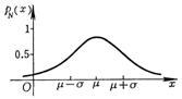
For a unimodal symmetrical distribution function, m = = ![]()
![]() (mean)
(mean)
For asymmetric unimodal distribution functions, m lies between and .![]()
![]()
[ Higher-order origin moment and central moment ] When r , the mathematical expectation (assuming existence) of the random variable and ( is called the r -order origin moment and the r -order central moment of the random variable, respectively, denoted as sum . In particular, it is the mean value, which is variance.![]()
![]()
![]()
![]()
![]()
![]()
![]()
![]()
1 ° If a continuous random variable has a distribution density of p(x) , then![]()
![]()
![]()
2 ° If it is a discrete random variable, its possible value is x k ( k = 1,2,...) , and P ( =x k ) =p k , then![]()
![]()
![]()
![]()
![]()
3 ° When r![]() , the mathematical expectation of the random variable and (assuming they exist) are called the r -order absolute origin moment and the r -order absolute central moment of the random variable, respectively. And there are similar formulas corresponding to 1 ° and 2 ° .
, the mathematical expectation of the random variable and (assuming they exist) are called the r -order absolute origin moment and the r -order absolute central moment of the random variable, respectively. And there are similar formulas corresponding to 1 ° and 2 ° .![]()
![]()
![]()
4 ° The origin moment and the central moment satisfy the following relationship ( r is a positive integer); ![]()
![]()
![]()
![]()
where is the binomial coefficient.![]()
[ Covariance and Correlation Coefficient ] Assuming that
both the mean and variance of the sum of random variables exist, then the covariance or Cov of the sum ( for![]()
![]()
![]()
![]()
![]()
![]()
![]() = E [(
= E [(![]()
![]() and the correlation coefficient is
and the correlation coefficient is![]()
![]()
![]() =
=
4.
Probability Generating Function Moment Generating Function Characteristic Function
[ Probability generating function of an integer-valued random variable ] If only random variables with non-negative integer values are taken, the mean of the random variable function is called the probability generating function of the random variable. Write P= ( =k ) =p k ( k= 0,1,2,...) , then the probability generating function is![]()
![]()
![]()
![]()
![]()
![]()
P ( ( -![]() 1
1![]()
set , then![]()
![]() (1) =E
(1) =E![]()
![]() (1) =E [
(1) =E [![]()
・・・・・・・・・・・・・・・・・・・・・・・・・・・・・・・・
P![]()
in turn have ![]()
![]()
[ Moment generating function ]
If it is a random variable, it is called the mean value of the random variable function![]()
![]()
![]()
is the moment generating function. If there is an origin moment of any order . . . ) , then![]()
![]()
![]()
![]()
![]()
1 ° If it is a discrete random variable, its possible values are x 1 , x 2 , · · · , then ![]()
![]()
![]()
2 ° If a continuous random variable has a distribution density of p ( x ), then ![]()
![]()
[ Characteristic function ] If it is a random variable, it is called
the mean value of the complex -valued random variable e![]()
![]()
![]() ( i = )
( i = )![]()
for the characteristic function. If there is an origin moment of any order ( k =1,2,...) , then![]()
![]()
![]()
![]()
![]()
![]() If it is a discrete random variable, its possible values are x 1 , x 2 ,..., P( , then
If it is a discrete random variable, its possible values are x 1 , x 2 ,..., P( , then![]()
![]()
![]()
2 ° If a continuous random variable has a distribution density of p ( x ) , then ![]()
![]()
[ Relationship between probability generating function, moment generating function and characteristic function ]
P ( e t )=![]()
P ( e it )=![]()
![]()
Five,
commonly used distribution functions
1. Commonly used discrete distributions
|
name notation |
Probability distribution and its domain parameter conditions |
mean |
variance |
probability generating function
|
moment generating function
|
Characteristic Function
|
icon |
|
|
binomial distribution
|
|
|
|
|
|
|
|
|
|
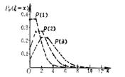
Poisson distribution
|
|
|
|
|
|
|
|
|
|
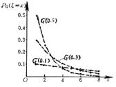
geometric distribution
|
|
|
|
|
|
|
|
|
|
Negative binomial distribution
|
|
|
|
|
|
|
|
|
|
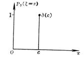
single point distribution
|
|
|
|
|
|
|
|
|
|
name notation |
Probability distribution and its domain parameter conditions |
mean |
variance |
probability generating function
|
moment generating function
|
Characteristic Function
|
icon |
|
|
log distribution
|
|
|
|
|
|
|
|
|
|
hypergeometric distribution
|
|
|
( for the hypergeometric function) |
|
||||


2. Commonly used continuous distribution
|
name notation |
Distribution Density and Its Definition Domain parameter conditions |
mean |
variance |
moment generating function
|
Characteristic Function
|
icon |
|
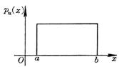
Uniform function
|
|
|
|
|
|
|
|
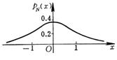
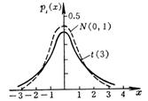
Standard normal distribution
|
|
0 |
1 |
|
|
|
|
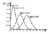
normal distribution
|
|
|
|
|
|
|
|
Rayleigh distribution
|
|
|
|
|
|
|
|
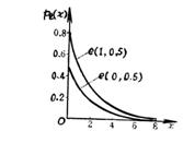
index distribution
|
|
|
|
|
|
|
|
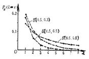
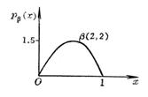
beta distribution
|
|
|
|
(Kummer function) |
|
|
|
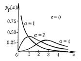
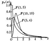
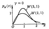
Gamma distribution
|
|
|
|
|
|
|
|
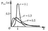
Lognormal distribution
|
|
|
|
|
|
|
|
|
n is a positive integer |
n |
2 n |
|
|
|
|
|
n is a positive integer |
0 ( n> 1) |
|
|
|
|
|
F distribution (degrees of freedom ( m,n ) ) F ( m,n ) |
|
|
|
(Kummer function) |
|
|
|
Wilbur distribution
|
positional parameters |
|
|
|
|
|
|
Cauchy distribution
|
|
does not exist |
|
|
||


6. The Law of Large Numbers and the Central Limit Theorem
[ Law of Large Numbers ]
1 ° Bernoulli's Theorem The frequency of random event A in n independent trials converges to the probability p of event A according to probability , that is, for any , ![]()
![]()
![]()
2 ° Independent random variables ... if (i) has a mean variance. Note E , )![]()
![]()
![]()
; or ( ii ) have the same distribution with finite mean E. then![]()
![]()
Convergence to the mean of random variables according to probability , that is, for any ,![]()
![]()
3 ° If the mean and variance of random variables with the same distribution are independent of each other , remember that ![]()
![]()
![]()
![]()
converges to the variance of the random variable according to the probability , that is, for any ,![]()
![]()
[ Central Limit Theorem ]
1 ° If the mean and variance of random variables with the same distribution are independent of each other , remember , then the random variable ![]()
![]()

Asymptotically follow the standard normal distribution N(0,1) , that is
2 ° under the condition of 1 ° , there is
or
Seven,
the use of the normal distribution table
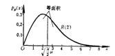
In practice, many random phenomena follow a normal distribution, or asymptotically follow a normal distribution with appropriate transformations. This manual accompanies the normal probability integral
table of values, and the integral
 ( K
( K![]()
![]()
Median and value correspondence table. Using them, the following problems can be calculated:![]()
![]()
1 ° The probability of a random variable following a standard normal distribution falling within the interval is ![]()
![]()
![]()
The one-sided probability is
(or from the values found in the value-to- value correspondence table ).![]()
![]()
![]()
![]()
2 ° known , determine the integral
![]()
in . by symmetry![]()
Find out from the value-to- value correspondence table , then .![]()
![]()
![]()
![]()
3 ° The probability that a random variable that follows a normal distribution falls within the interval is ![]()
![]()
![]()
![]()
The one-sided probability is
![]()
![]()