§ 2 Mathematical and statistical methods
1.
Estimation of overall parameters
1. Population (maternal body) and sample (sub-sample)
When studying a problem, all possible observations of its objects are called the population (or matrix), denoted by . A part of the sample taken from the population is called a sample (or subsample) of the population. The number of samples in a sample is called the size (or capacity) of the sample. , can be considered as a large sample, otherwise it is called a small sample.![]()
![]()
![]()
![]()
Mathematical statistical method is a scientific method to understand and judge the statistical characteristics of the population through samples by applying the results of probability theory.
2. Comparison table between the number of sample characteristics and the overall numerical characteristics
|
name |
number of sample features |
Overall Numerical Characteristics |
|
mean |
|
|
|
variance |
|
|
|
standard deviation |
|
|
|
Coefficient of variation |
|
|
|
skewness coefficient |
|
|
|
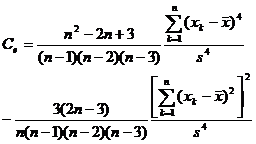
kurtosis coefficient |
|
|
Note that when 1 ° is larger, take ![]()
![]()
![]()
(Sometimes this is called the sample variance, and the one in the table is called the sample corrected variance)![]()
![]()


The 2 ° sample characteristic coefficients are also:
sample order origin moment![]()
![]()
Sample order central moment ![]()
Sample median (sample size n is odd) ![]()
sample mean
![]()
Very poor sample
![]()
3. Point estimation of population parameters
Note that x 1 , x 2 ,..., x n is a sample taken from the population, and the number of features of the sample can be used to estimate the numerical characteristics of the population. There are two commonly used methods:![]()
[ Moment method ] The moment method uses the r -order moment of the sample as an estimate of the overall r -order moment. Specific steps are as follows:
The set distribution function contains k parameters (the values of which are unknown), denoted as . The assumed origin moments of order k exist, and they are naturally functions of, i.e.![]()
![]()
![]()
![]()
![]()
![]() ( r= 1,2,... ,k )
( r= 1,2,... ,k )
Consider a sample of the population to make the r -order moment of this sample , that is![]()
![]()
![]() =
=![]()
Then solve the system of equations
![]() ( = (
( = ( ![]()
![]() r=1,2,...,k)
r=1,2,...,k)
The obtained solution is
![]()
Use separately as the valuation.![]()
![]()
[ Maximum Likelihood Method ] Assuming that the overall distribution is continuous, the distribution density function is , where is the unknown parameter to be estimated. For a given function that maximizes the function , use them as estimates respectively.![]()
![]()
![]()
![]()
![]()
![]()
Since ln reaches its maximum value at the same point ( ), the function is introduced![]()
![]()
![]()
L ( )= ![]() ln = )
ln = )![]()
![]()
![]()
It is called the likelihood function. Just solve the system of equations
![]() ( i= 1,2,..., k )
( i= 1,2,..., k )
The required values can be determined from them, which are called the maximum likelihood estimates of the parameters, respectively.![]()
![]()
If the overall distribution is discrete, it is enough to take the above likelihood function as .![]()
![]()
Example of parameter estimation of a normal population, assuming that the population is known to follow a normal distribution N ( , but the parameters are unknown. Now use the maximum likelihood estimation of n observations of the population x 1 , x 2 ,..., x n value. ![]()
![]()
![]()
The solution is because the distribution density function of the population is

Therefore, the likelihood function is
![]()
solve system of equations

have to
![]()
![]()
It is easy to verify that the maximum value is indeed taken. So they are respectively the maximum likelihood estimates of .![]()
![]()
![]()
[ Criteria for judging whether the valuation is good or bad ]
1 ° unbiasedness if the parameter estimates x 1 , x 2 ,..., x n ) satisfy the relation ![]()
![]()
![]()
is called an unbiased valuation.![]()
![]()
2 ° validity if and are both unbiased estimates of the parameters . ![]()
![]()
![]()
![]()
is said to be more effective. Further, if the sample size n is fixed , the unbiased estimate of the minimum value is called the efficient estimate.![]()
![]()
![]()
![]()
![]()
3 ° Consistency If for any given positive number , there is always ![]()
![]()
The valuations are said to be consistent.![]()
![]()
It is easy to see from Chebyshev's inequality (see § 1, 3) that when
![]()
A consistent valuation of yes when it is established.![]()
![]()
![]()
In practice, this sufficient condition is often applied to verify whether it is a consistent estimate.![]()
![]()
example
|
Overall distribution |
unknown population parameter |
Overall parameter estimates |
unbiased |
validity |
consistency |
|
|
|
|
Have Have Have Have Have Have Have |
Have Have Have Have |
Have Have Have Have Have Have |
4. Frequency distribution of samples
The frequency distribution more completely reflects the change law of the experimental data. The steps to build a frequency distribution (let the samples be x 1 , x 2 ,..., x n ) are:
( 1 ) Find the maximum and minimum values, and obtain the range .![]()
( 2 ) Grouping according to the sample size, usually large samples are divided into 10-20 groups , small samples are divided into 5-6 groups, and then the group distance c is determined according to the number of groups k and the range R , if the grouping is equidistant, then c .![]()
![]()
( 3 ) Determine the sub-point (often take one bit higher than the precision of the original data).
( 4 ) Count the frequencies of each group .![]()
( 5 ) Calculation frequency![]()
( 6 ) Draw a histogram (the sub-point is the abscissa, and the ratio of the frequency to the group distance is the ordinate).
( 7 ) If the variable is continuous, a smooth curve is drawn to approximate the overall distribution.
5. Interval estimation of population parameters
[ Principle of Small Probability ]
In an experiment, an event with a small probability (close to zero) is considered to be an event that is actually impossible; and an event with a probability close to 1 is considered to be an event that is actually inevitable.
[ Confidence interval and significance level ] When performing interval estimation (that is, estimating the value range of the parameter) for
a population parameter (eg ), if for a pre-given small probability , an interval ( ) can be found such that![]()
![]()
![]()
![]()
![]() = 1 -
= 1 -![]()
Then the interval ( ) is called ![]() the confidence interval of the parameter , and the sum is called the confidence limit (or critical value); the sum is called the negative field; the probability is called the significance level, and 1 - is called the confidence level (or confidence probability).
the confidence interval of the parameter , and the sum is called the confidence limit (or critical value); the sum is called the negative field; the probability is called the significance level, and 1 - is called the confidence level (or confidence probability).![]()
![]()
![]()
![]()
![]()
![]()
![]()
[ Table of interval estimates for population parameters ]
assuming that the population follows a normal distribution ) . For the pre-given significance level , the mean and standard deviation s of a sample x 1 ,
x 2 ,..., x n can be used to estimate the confidence interval of the mean and variance of the population, and the mean and standard of the two samples can also be used. difference to estimate the confidence interval for the difference between the two population means.![]()
![]()
![]()
![]()
![]()
![]()
![]()
![]()
![]()
![]()
![]()
|
Sample situation |
Confidence intervals for population parameters or |
Determination of and in relation to confidence intervals |
|
Large sample known population variance
|
|
Check the normal distribution table |
|
Large sample Population variance unknown |
|
Ditto |
|
Small sample known population variance
|
|
Ditto |
|
Small sample Population variance unknown |
|
Look up the t distribution table (with n -1 degrees of freedom ) |
|
known two populations variance |
|
Check the normal distribution table |
|
The variance of the two populations unknown |
in the formula |
Look up the t distribution table (degrees of freedom are n 1 + n 2 -2 ) |
|
Small sample known population mean |
|
Check distribution table (with n degrees of freedom ) |
|
Small sample The population mean is unknown |
|
Check distribution table (with n |
|
Small sample mean of the two populations with variance unknown |
|
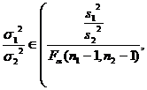
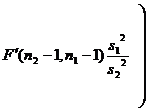
Look up the F distribution table (degrees of freedom are
Check distribution table (The degrees of freedom are ( n 2 _ -1, n 1 –1) ) |


