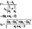
2. Statistical Hypothesis Experiment
![]()
![]()
1. Steps of Statistical Hypothesis Testing
It is assumed that the population has certain statistical properties (such as having a certain parameter, or following a certain distribution, etc.), and then testing whether the hypothesis is credible. This method is called statistical hypothesis testing (or hypothesis testing). The steps are as follows:
For example , if the average strength of a certain product is known in kilograms, the production method is changed, and parts are randomly selected to calculate kilograms and kilograms. Q Does the change in the production method have a significant effect on the strength?
![]()
![]()
![]()
![]()
|
Statistical Hypothesis Testing Steps |
Process analysis |
|
( 1 ) Suppose H 0 ( 2 ) Select statistics and clarify their distribution ( 3 ) gives the significance level ( 4 ) Find out the confidence limit ( 5 ) Calculate the statistic u ( 6 ) Statistical inference At that time , accept H 0 At that time , negating H 0 |
H 0 : ( is the overall mean after the production method has been changed)
Depend on Check the normal distribution table to get K 0.025 =1.96
due to Therefore, it is believed that H 0 , with a significance level of 5 % , the change in the manufacturing method is considered to have no significant effect on the strength of the product. |
2. Statistical hypothesis test table for normal population parameters
For large samples, no matter the population follows the even distribution, according to the central limit theorem, it can be considered that the sample mean asymptotically follows the normal distribution. Therefore, statistical hypothesis testing of population parameters was performed using the " u- test method " described below.![]()
In the table is the given significance level, which is the sample mean, and s is the sample standard deviation.![]()
![]()
|
name |
Condition and inspection purpose |
Assumption |
Statistics and their distribution |
Negative domain |
Determination of confidence limits |
|
check test Law |
Given the population variance , test whether the mean of the population is equal to (or less than or greater than) a known constant |
|
|
|
|
|
Two population variances are known to be equal
Compare the two population means and |
|
|
|
|
|
|
Condition and inspection purpose |
Assumption |
Statistics and their distribution |
Negative domain |
Determination of confidence limits |
|
|
Two population variances are known Compare two population means
|
|
|
|
|
|
|
check test Law |
Population variance unknown, test whether the population mean is equal to (or less than or greater than) a known constant |
|
|
|
|
|
Two populations are known to have the same variance (but the value is unknown), compare the sum of the means of the two populations . |
|
|
|
|
|
|
check test Law |
Given the population mean , test whether the population variance is equal to (or less than or greater than) a known constant . |
|
|
|
or
|
|
The population mean is unknown, test whether the population variance is equal to (or less than or greater than) a known constant . |
|
|
or
|
or |
|
|
check test Law |
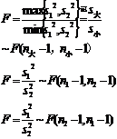
The mean and variance of the two populations are unknown, and the variances of the two populations are compared |
|
|
|
|
3. Statistical hypothesis testing of the overall distribution function
Let be a known type of distribution function, be a parameter (known or partially known), be a sample of the population, and be a hypothesized distribution function , and perform statistical hypothesis testing in two cases.![]()
![]()
![]()
![]()
![]()
![]()
All parameters of 1 ° are known to divide the real axis into m disjoint intervals:![]()
![]()
![]() which is understood to be . Let the theoretical frequency be
which is understood to be . Let the theoretical frequency be![]()
![]()
![]()
![]() The number of samples that fall in the interval is (empirical frequency), then the statistic
The number of samples that fall in the interval is (empirical frequency), then the statistic![]()
![]()
![]()
![]()
Following a distribution with m![]() degrees of freedom, the hypothesis can be tested by applying the test method
degrees of freedom, the hypothesis can be tested by applying the test method![]()
H 0 : F ( x ) =F 0 ( x )
Is it credible.
All or part of the parameters of 2 ° F 0 ( x ) are unknown. If there are l parameters unknown, the maximum likelihood method (this section, 1, 3 ) can be used to determine the estimates of these l parameters. As the corresponding parameter, then the theoretical frequency can be calculated in the case of 1 ° , and then the empirical frequency can be calculated, then the statistic ![]()
![]()
![]()
![]()
When n is large, it follows a distribution with degrees of freedom. Hypotheses can be tested by applying tests![]()
![]()
H 0 : F ( x ) =F 0 ( x )
Is it credible.
4. Statistical hypothesis test for whether two samples are from the same distribution population
[ Symbol test method ] This method is simple and intuitive, and does not require an understanding of the distribution law of the test quantity. It is often used to test whether the degree of fluctuation is the same and whether there is an obvious change in the production status.
The symbols " + " , " - " and " 0 " are used to indicate that the data of A is larger, smaller and equal than that of B respectively, and , and are used to indicate the number of occurrences of " + " , " - " and " 0 ". Statistical hypothesis testing step use case description is as follows:![]()
![]()
![]()
Example A and B analyze the content of a certain component in the same substance and obtain the following table
|
First Second symbol |
14.7 15.0 15.2 14.8 15.5 14.6 14.9 14.8 15.1 15.0 14.6 15.1 15.4 14.7 15.2 14.7 14.8 14.6 15.2 15.0 + - - + + - + + - 0 |
|
First Second symbol |
14.7 14.8 14.7 15.0 14.9 14.9 15.2 14.7 15.4 15.3 14.6 14.6 14.8 15.3 14.7 14.6 14.8 14.9 15.2 15.0 + + - - + + + - + + |
Are there any significant differences in the results of the two analyses ?
|
Statistical Hypothesis Testing Steps |
Process analysis |
|
(1) Suppose H 0 (2) Statistics (3) Give the significance level (4) Find out the confidence limit (5) Calculate statistics (6) Statistical inference At that time , accept H 0 At that time , negating H 0 |
Assume that the two analysis results have the same distribution function r= min { n + , n - } a = 10% Check the symbol inspection table ( see next page ), by N=n + + = 12+7=19, a = 10% , the negative domain is . because r= 7>5 =r 10% Therefore, accepting H 0 means that there is no significant difference in the analysis results of A and B with 10% reliability . |
Symbol Checklist _
|
N |
1 5 10 25 ( % ) |
N |
1 5 10 25 ( % ) |
N |
1 5 10 25 ( % ) |
|
1 2 3 4 5 6 7 8 9 10 11 12 13 14 15 16 17 18 19 20 twenty one twenty two twenty three twenty four 25 26 27 28 29 30 |
0 0 0 0 0 0 1 0 0 1 0 0 1 1 0 1 1 2 0 1 1 2 0 1 2 3 1 2 2 3 1 2 3 3 1 2 3 4 2 3 3 4 2 3 4 5 2 4 4 5 3 4 5 6 3 4 5 6 3 5 5 6 4 5 6 7 4 5 6 7 4 6 7 8 5 6 7 8 5 7 7 9 6 7 8 9 6 7 8 10 6 8 9 10 7 8 9 10 7 9 10 11 |
31 32 33 34 35 36 37 38 39 40
41 42 43 44 45 46 47 48 49 50 51 52 53 54 55 56 57 58 59 60 |
7 9 10 11 8 9 10 12 8 10 11 12 9 10 11 13 9 11 12 13 9 11 12 14 10 12 13 14 10 12 13 14 11 12 13 15 11 13 14 15 11 13 14 16 12 14 15 16 12 14 15 17 13 15 16 17 13 15 16 18 13 15 16 18 14 16 17 19 14 16 17 19 15 17 18 19 15 17 18 20 15 18 19 20 16 18 19 21 16 18 20 21 17 19 20 22 17 19 20 22 17 20 21 23 18 20 21 23 18 21 22 24 19 21 22 24 19 21 23 25 |
61 62 63 64 65
66 67 68 69 70 71 72 73 74 75 76 77 78 79 80 81 82 83 84 85
86 87 88 89 90 |
20 22 23 25 20 22 24 25 20 23 24 26 21 23 24 26 21 24 25 27 22 24 25 27 22 25 26 28 22 25 26 28 23 25 27 29 23 26 27 29 24 26 28 30 24 27 28 30 25 27 28 31 25 28 29 31 25 28 29 32 26 28 30 32 26 29 30 32 27 29 31 33 27 30 31 33 28 30 32 34 28 31 32 34 28 31 33 35 29 32 33 35 29 32 33 36 30 32 34 36 30 33 34 37 31 33 35 37 31 34 35 38 31 34 36 38 32 35 36 39 |
[ Note ] The numbers in the table represent the sign limits corresponding to the sign and N and the significance level .![]()
![]()
[ Rank sum test method ] This method has higher accuracy than the symbol test method , can better utilize the information provided by the data , and does not require the data to be "paired" . The steps and use cases are described as follows :
For example, a life test is carried out on a product made of two materials, A and B , and it is found that
A 1610 1650 1680 1700 1750 1720 1800
B 1580 1600 1640 1640 1700
Is there any significant difference in the impact of the two materials on product quality ?
Solution Arrange the above data into the following table from small to large :
|
rank |
1 2 3 4 5 6 7 8 9 10 11 12 |
|
First Second |
1610 1650 1680 1700 1720 1750 1800 1580 1600 1640 1640 1700 |
The rank in the first row in the above table represents the ordinal number arranged from small to large. There are 1700 A and B data , and they are ranked in two ordinal positions of 8 and 9. The rank is taken according to the average rank .![]()
|
Statistical Hypothesis Testing Steps |
Process analysis |
|
( 1 ) Suppose H 0 ( 2 ) Statistics ( 3 ) gives the significance level ( 4 ) Find out the confidence limit ( 5 ) Calculate statistics ( 6 ) Statistical inference At that time , accept H 0 When or , negate H 0 |
Assuming no significant difference in the impact of the two materials on product life T = sum of ranks for the group with the smaller number of samples
Check the "rank sum test table" (see next page), parameters n 1 =5, n 2 =7 ( n 1 and caps (i.e. negative domains or T= 1+2+4+5+8.5=20.5 (rank sum of group B) Because , so negate H 0 , that is, with 5 % , think that the influence of the two materials on the product life is significantly different |
rank sum test table
|
n 1 |
n 2 |
|
|
n 1 |
n 2 |
|
|
n 1 |
n 2 |
|
|
n 1 |
n 2 |
|
|
n 1 |
n 2 |
|
|
|
2 2 2 2 2 2 2 2 2 2 2 2 3 3 3 3 3 |
4 5 6 6 7 7 8 8 9 9 10 10 3 4 4 5 5 |
3 3 3 4 3 4 3 4 3 4 4 5 6 6 7 6 7 |
11 13 15 14 17 16 19 18 twenty one 20 twenty two twenty one 15 18 17 twenty one 20 |
3 3 3 3 3 3 3 3 3 3 4 4 4 4 4 4 4 |
6 6 7 7 8 8 9 9 10 10 4 4 5 5 6 6 7 |
7 8 8 9 8 9 9 10 9 11 11 12 12 13 12 14 13 |
twenty three twenty two 25 twenty four 28 27 30 29 33 31 25 twenty four 28 27 32 30 35 |
4 4 4 4 4 4 4 5 5 5 5 5 5 5 5 5 5 |
7 8 8 9 9 10 10 5 5 6 6 7 7 8 8 9 9 |
15 14 16 15 17 16 18 18 19 19 20 20 twenty two twenty one twenty three twenty two 25 |
33 38 36 41 39 44 42 37 36 41 40 45 43 49 47 53 50 |
5 5 6 6 6 6 6 6 6 6 6 6 7 7 7 7 7 |
10 10 6 6 7 7 8 8 9 9 10 10 7 7 8 8 9 |
twenty four 26 26 28 28 30 29 32 31 33 33 35 37 39 39 41 41 |
56 54 52 50 56 54 61 58 65 63 69 67 68 66 73 71 78 |
7 7 7 8 8 8 8 8 8 9 9 9 9 10 10 |
9 10 10 8 8 9 9 10 10 9 9 10 10 10 10 |
43 43 46 49 52 51 54 54 57 63 66 66 69 79 83 |
76 83 80 87 84 93 90 98 95 108 105 114 111 131 127 |
[ Note ]
The header indicates the number of data in the two groups; and are the lower and upper limits of the rank sum, respectively. The corresponding rank and upper and lower limits are represented by bold numbers, and the corresponding rank and upper and lower limits are represented by ordinary fonts.![]()
![]()
![]()
![]()
![]()
3. Analysis of variance
Analysis of variance is a method of analyzing experimental (or observational) data. The basic problem it solves is to clarify the influence of various factors related to the research object and the interaction between various factors on the object through data analysis. The objects it studies are assumed to follow a normal distribution.
[ One-way ANOVA ] considers the influence of different levels of a factor A on the object under investigation. Test for k different levels A i of A (their distributions are tested to obtain test data ; n k ) assuming (although the value is unknown), test whether the mean of the test results of each A i is significantly different. The inspection steps are as follows:![]()
![]()
![]()
![]()
![]()
( 1 ) Assumption![]()
( 2 ) Select statistics and clarify their distribution
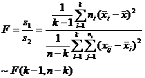
in the formula
![]()
![]()
( 3 ) gives the significance level![]()
( 4 ) The confidence limit can be found from the F distribution table (degree of freedom is ( k -1, n - k ) ) , which satisfies![]()
![]()
( 5 ) List calculation statistics.
|
Grading |
Test data x ij |
n i |
|
|
|
|
|
|
A 1 A 2
A k |
|
n 1 n 2 n k |
|
|
|
|
|
|
|
|
|
|
|
|
|
|
|
mark |
|
|
|
||||
( 6 ) One-way ANOVA table
|
variance source |
sum of square |
degrees of freedom |
mean square |
Statistics |
confidence limits |
statistical inference |
|
Between groups s |
|
k n |
|
|
|
At that time , accept H 0 At that time , negating H 0 |
|
sum |
|
n |
|
|
|
|
Explanation: If the value of 1 ° is larger, take it as a constant, then use it instead to carry out the above calculation, and the analysis result will not change. 2 ° The between - group variance S1 reflects the systematic error caused by different levels of factor A , while the within-group variance S2 is the within - group difference caused by random factors. If the effects of different factors A i are similar, the ratio of the between-group variance to the within-group variance is small, then it can be considered ; if the effects of different factors A i are significantly different, the ratio of the between-group variance to the within-group variance is larger, it cannot be considered .![]()
![]()
![]()
![]()
![]()
![]()
[ Two-way ANOVA ]
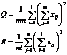
Consider the influence of two factors A and B. A is divided into l grades A 1 , A 2 , ··· , A l . B is divided into m grades B 1 , B 2 , ··· , B m under the condition of two factors A i j (that is, A i and B j are required to make lm kinds of cooperation in each test) for n trials, get lmn data . the assumed distribution , testing the effect of A or![]()
![]()
![]()
![]() Whether the effect of B or the effect of B has a significant effect on the test results, respectively. The inspection steps are as follows:
Whether the effect of B or the effect of B has a significant effect on the test results, respectively. The inspection steps are as follows:![]()
( 1 ) Hypothesis H 0 : The corresponding effect ( A or B or ) has no significant effect on the test results.![]()
( 2 ) Select statistics and clarify their distribution


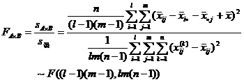
where F A , F B
and represent the effect of factor A , the effect of B and the interaction of factors A and B , respectively, and![]()
![]() ,
,![]()
![]()
![]()
( 3 ) gives the reliability .![]()
( 4 ) Find out the confidence limits . When the degrees of freedom are , then![]()
![]()
![]()
![]()
( 5 ) List calculation statistics (Table 1 and Table 2 ).
Table 1
|
A |
B |
test results |
|
|
|
|
|
A 1 |
B 1 B 2
Bm |
|
|
|
|
|
|
|
|
|
|
|
|
|
|
A l |
B 1 B 2
Bm |
|
|
|
|
|
|
|
|
|
|
|
|
|
mark |
|
|
|
||
Table
2
|
|
B 1
B 2 ... B m |
|
|
|
A 1 A 2 A l |
x 11
x 12 ... x 1 m x 21
x 22 ... x 2 m
x l 1
x l 2 ... x lm |
|
|
|
|
|
|
|
|
|
|
|
|
( 6 ) Two-way ANOVA table
|
variance source |
sum of square |
degrees of freedom |
mean square
|
Statistics |
confidence limits |
statistical inference |
|
A 's effect B 's effect |
S A = Q S B =R |
l m |
|
|
|
when
|
|
role random action |
S A B T– Q + P S false = W |
( l lm ( n |
|
|
|
when
|
|
total flat Fang He |
S |
lmn |
|
|
|
|
When the interaction of the two factors A and B is not significant, S A B![]() and S are mistakenly mixed together. At this time, if only one experiment is performed under the condition (ie n= 1 ), the measured experimental data is x i j , record
and S are mistakenly mixed together. At this time, if only one experiment is performed under the condition (ie n= 1 ), the measured experimental data is x i j , record![]()

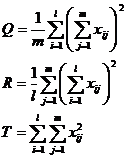
but
![]()
At this time, the statistics and distribution of factor A and factor B are
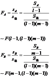
The calculation process and analysis of variance are the same as before.
[ Analysis of variance by systematic grouping ] The method of grouping by system is often used for investigation. For example, when a county is surveyed, several communes are selected, each commune also selects several brigades, and each brigade selects several production teams. This approach is called system grouping.
ANOVA for systematic grouping is different from multivariate ANOVA. For example, in the two - way ANOVA, the factors A and B are parallel, but in the ANOVA of the systematic grouping , A and B are not parallel . l , and then in each group A i are grouped by factor B into B i 1 , B i 2 ,..., B im . However, the method of analysis is similar.
Suppose n times of tests are made under the conditions of factor A i and factor B ij , and the test data is , and the inspection steps are as follows:![]()
( 1 ) Hypothesis H 0 : Under the condition, the effect of factor A (or B ) is not significant. ![]()
( 2 ) Select statistics
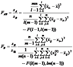
where F AB and F B represent the significance of the influence of factor A and factor B , respectively, and
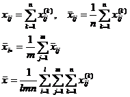
( 3 ) gives the reliability . ![]()
( 4 ) Find out the confidence limits . When the degrees of freedom are![]()
![]()
![]()
![]()
(5) List calculation statistics
|
|
|
Test result x ij (k) |
|
|
|
|
|
|
|
A 1 |
B 11 B 12
|
|
x 11 x 12 x 1 m |
|
|
|
|
|
|
|
|
|
|
|
|
|
|
|
|
A l |
B l 1 B l2
B l m |
|
x 11 x 12 x 1 m |
|
|
|
|
|
|
|
|
|
|
|
|
|||
|
mark |
|
|
|
|
||||
( 6 ) System grouping variance analysis table
|
source of variance |
sum of square |
degrees of freedom |
mean square |
Statistics |
confidence limits |
statistical inference |
|
The role of A The role of B random action |
S A = QP S B = TQ S false = W - T |
l- 1 l ( m- 1) lm ( n- 1) |
|
|
|
At that time, H 0 was accepted , and the corresponding factors were considered to be insignificant; At that time , it was negative , and the corresponding factors were considered to have a significant impact. |
|
total sum of squares |
|
lmn |
|
|
|
|


