§ 2    Interpolation formula

 

1. The        unequal distance node interpolation formula ( difference quotient interpolation polynomial )

 

The n+ 1 nodes of the known univariate function f(x) and their corresponding function values ​​are for the interpolation interval  

At any point x , the function value f(x) can be calculated by the following difference quotient interpolation polynomial :

where are the first-order difference quotient, the second-order difference quotient, ... , the n -order difference quotient, respectively. Calculations can be performed column by column from left to right as follows:

 

		first order difference quotient	second order difference quotient	third order difference quotient	…	n -order difference quotient
					…

 

  The first order difference quotient in the table

                                         

  second order difference quotient

                                   

  third order difference quotient

                             

  ………………………………

  n -order difference quotient

                        

  Remainder in Difference Quotient Interpolating Polynomial

             

                         

  The remainder can also be written as

             

The n+ 1 order difference quotient expressed in the formula . It is convenient to use such remainders for some values ​​of the function given by the measurement or for functions whose analytical expressions are more complex.

The difference quotient interpolation polynomial clearly satisfies

                   

The specific interpolation calculation steps are as follows :

First , calculate the difference quotient of each order by the difference quotient table, and then calculate a point a in the given interpolation interval , then

 

   

2.        Isometric node interpolation formula ( difference formula )

 

[ Forward difference and backward difference ]   Known function f(x) at equidistant nodes

                     

value of

                          

The difference is calculated as follows

first order difference                        

second order difference      

……………………

k -order difference  

                                           

The symbol is called forward difference. In addition, symbols can be introduced , which are defined as

             

The symbol is called backward differencing.

   The relationship between forward difference and backward difference is

                       

  [ Difference table ]    

x	y
						B

  [ Newton's first interpolation formula ( Newton's forward interpolation formula )]

  node is the step size)                

  Interpolation point ( 0 < u< 1 )                  

  Interpolation formula  

            

  remainder _            

where is the binomial coefficient.

  The applicable range is usually used to calculate the function value near the start point of the interpolation interval . 

  [ Newton's second interpolation formula ( Newton's backward interpolation formula )]

  Node ( h > 0)             

  interpolation point   

  Interpolation formula 

           

  remainder _            

in the formula

            

When using backward differential

            

 

  Scope is typically used to compute function values ​​near the endpoints of an interpolated interval . 

  [ Sterling interpolation formula ]

node            

interpolation point 

Interpolation formula 

          

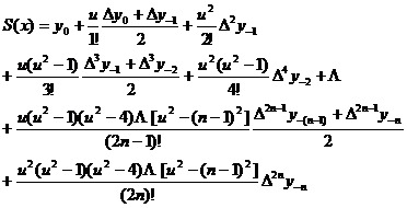
remainder _     

                           

Scope is typically used to compute function values ​​around the midpoint of an interpolated interval. generally when 

use this formula.

Note that the number of nodes used each time is an odd number. 

[ Bezier interpolation formula ]

node             

    interpolation point 

Interpolation formula 

   

       

       

       

       

   

remainder _          

    

                                    

     The applicable range is usually used to calculate the function value near the midpoint between two adjacent nodes. This formula is generally used when . 

     Precautions The number of nodes used each time is an even number. 

     At the time , the interpolation formula was particularly simple :

     

     

     It shows that when the difference method is used for interpolation, it is not that the more items the more accurate the result, the more accurate the result is. It is not difficult to see that the linear interpolation method is only a special case of the difference method ( taking the first-order difference ) . 

 

3. Lagrangian Interpolation Polynomial

  

  [ Lagrangian interpolation formula ] Given   n+ 1 nodes of a univariate function and their corresponding function values , for any point x in the interpolation interval, the following Lagrangian interpolation polynomial can be used to calculate the function value:

           

here            

Especially for equidistant nodes , we have

     

in the formula         

   [ Etkin step-by-step calculation method ] Knowing that, to find the value   of the Lagrangian polynomial at any point a in the interpolation interval, the calculation can be performed column by column from left to right according to the following table.

						…
						…

The table represents the first-order interpolation polynomial used as a node; the first-order interpolation polynomial for the node is; the k -order interpolation polynomial for the node is generally represented . Each column after the fourth column from the left in the table is the value of the corresponding interpolation polynomial at point a , and there is the following relationship between them :

                  

                

       ……………………………………………………

       

    When using Lagrangian interpolation polynomial to calculate the value of a certain point a , each additional node must be recalculated according to the formula, and the Etkin step-by-step calculation method avoids this shortcoming.

 

Four cubic spline ( Spline ) interpolation formula

 

A spline function is a method of approximating a function.

[ Cubic spline function ] Known   n points on the plane , these points are called type-valued points, which are called nodes.

If the function S(x) satisfies the following three conditions :

( i ) ;

( ii ) S(x) is a cubic polynomial in each interval ;

( iii ) S(x) has continuous first and second derivatives over the entire interval ;

Then S(x) is called a cubic spline function through n points.

A cubic spline function S(x) exists and is unique if the function S(x) satisfies any of the following boundary conditions ( additional conditions at both ends ) :

( a ) The first derivative ( one-sided derivative ) of the function at both ends of the interval is known, that is, the sum is a known number.

( b ) The second derivative of the function at both ends of the interval is zero, ie .

( c ) The function is periodic and satisfies .

[ Expression form of cubic spline function ]

 The form S(x) with the second derivative as a parameter is expressed over each interval as  

                                     

where is the undetermined parameter, but is the first-order difference quotient of , and is the first-order difference quotient, that is

                               

                              

 The function S(x) thus defined satisfies the conditions (i) , (ii) on the interval . If the choice is made such that S(x) has a first-order continuous derivative on , then S(x) has a second-order continuous derivative on , and

                                   

Using the continuity and boundary conditions of the first derivative of S(x), a certain set of algebraic equations can be given.

(1)  The case where the boundary condition is ( a )

Under condition ( a ) , the following equations are solved

 

where is the first-order difference quotient ( same as before ) , and the sum is the given boundary condition.

Represented by a matrix

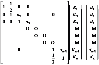
in the formula                           

                

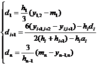
At that time , the solution was

     

(2)  The case where the boundary condition is ( b )

Under condition ( b ) , it is solved by the following system of equations:

           

                                     

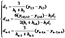
Represented by a matrix

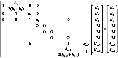
in the formula

                     

              

At that time , the solution was

             

  The form S(x) with the first derivative as a parameter is expressed over each interval as

      

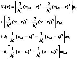
where is the parameter to be determined. The function S(x) defined in this way satisfies the conditions ( i ) and ( ii ) of the cubic spline function on the interval , and S(x) has a continuous first-order derivative on the interval, and at the same time

                                            

    Sometimes it is expressed as:

       

in the formula , and the same as the definition before.

A definite system of algebraic equations can be given according to the continuous second-order derivatives and boundary conditions on .

(1)    The case where the boundary condition is

Under the conditions , the following equations are satisfied

             

remember , gotta

           

It can be rewritten as

                  

in

         

From this we get   

                               

( 2 ) the case where the boundary condition is ( b )

Under condition ( b ) , the following equations are satisfied

               

where is the first-order difference quotient.

when and when ,  

                      

where , while recursively obtained by the following formula

   

                

   

         

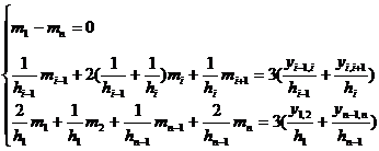
( 3 ) The case where the boundary condition is ( c )

Under condition ( c ) , the following equations are satisfied :

              

 

5. Other interpolation formulas

 

[ Univariate three-point interpolation formula ] Knowing the value of the   univariate function y=f(x) on n nodes , for any point x in the interpolation interval, the function value can be approximately calculated according to the following formula

 

where are the three known nodes closest to x .

[ Binary interpolation formula ] It is known   that the node of the first independent variable of the bivariate function is , the node of the second independent variable is , and the function value on the corresponding node is . Then for the argument value that is not a node, the function value can be approximated by the following formula

                                ( 1 )

                               ( 2 )

( 2 ) are the three nodes where the first argument is closest to x , and are the three nodes where the second argument is closest to y .

[ Hermitian Interpolation Formula with Derivative ] Knowing that the value of the   function y=f(x) and its derivative at n nodes is and , then for any point x in the interpolation interval, the function value can be calculated as follows

 

in the formula

     

     

remainder

     

where is a point in an interval [ a, b ] that contains all nodes .

It is easy to know that in the formula is a polynomial whose degree does not exceed and satisfies .