§ 4 Smoothing method of experimental curve
1. Smoothing of experimental curves and smoothing of observed values
The experimental data is represented as some discrete points on the coordinate plane. It is often too rough to directly use the polyline connecting these observation points in sequence to reflect the change of the function, so it is necessary to give a smooth experimental curve. It is usually required that the residual sum of squares of this experimental curve and the observed data be the smallest.
The experimental curve smoothing method is to smooth the observation results, eliminate the external interference and influence, and let the smoothed observation value fall on a smooth curve.
2. Linear moving average method
For the independent variable x , the experimental observation data is as follows :![]()
|
x |
|
|
y |
|
so that the above data becomes![]()
|
t |
-i |
|
|
|
Corrected value with the following method : take a definite positive integer n such that at least one holds. When and at the same time, choose such that![]()
![]()
![]()
![]()
![]()
![]()
From this we get

So the time-corrected formula![]()
![]()
When it is not established at the same time, it is selected such that![]()
![]()
![]()
In the formula, t takes the 2 n +1 integer values closest to i in [0, m ] . For these 2 n +1 t values, the revised formula is also obtained
![]()
Especially in the above two cases, let t = 0 , the correction value obtained![]()
![]()
For example, take n = 1. At that time![]()
![]()
And when i = 0 , it should be satisfied![]()
![]()
find out
![]()
When i = m , through the transformation , it can be known that we should take![]()
![]()
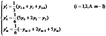
[ Take three-point moving average ] ( ie n = 1 )
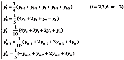
[ Take five-point moving average ] ( ie n = 2 )
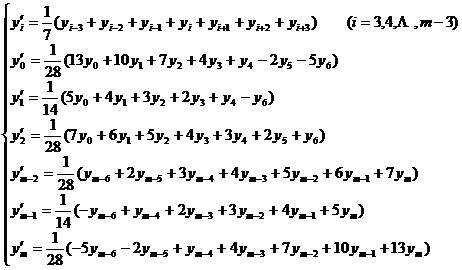
[ Take a seven-point moving average ] ( ie n = 3 )
The above correction value can also be expressed by a difference. First make a difference table according to the method in § 2 of this chapter
|
x |
Y |
|
|
|
|
|
|
|
|
|
|
|
|
|
|
|
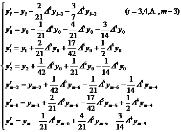
Then the correction value is expressed by difference as![]()
![]()
( i )
When n = 1 ( that is, taking a three-point moving average ) ,
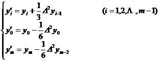
( ii ) When n = 2 ( that is, taking a five-point moving average ) ,
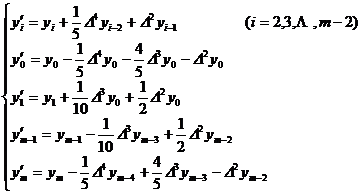
( iii ) When n = 3 ( that is, taking a seven-point moving average ) ,
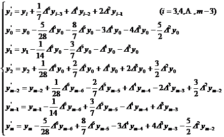
3. Moving average method of quadratic parabola
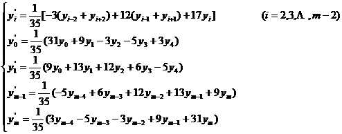
Following the notation of the previous paragraph , ![]() the correction value is taken as the quadratic parabola equation
the correction value is taken as the quadratic parabola equation![]()
![]() (1)
(1)
The coefficients a, b and c in the formula should be such that
![]()
In the formula, t takes the 2 n +1 integer values closest to i in [0, m ] . When both are established, the coefficients a, b, and c satisfy the following equations :![]()
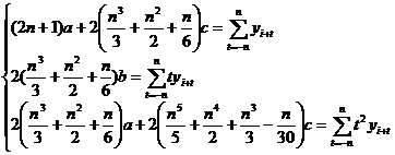
Solve a,b,c from this and substitute it into ( 1 ) to get the corrected value .![]()
![]()
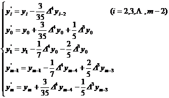
[ Take five-point moving average ] ( ie n = 2 )
or expressed by difference
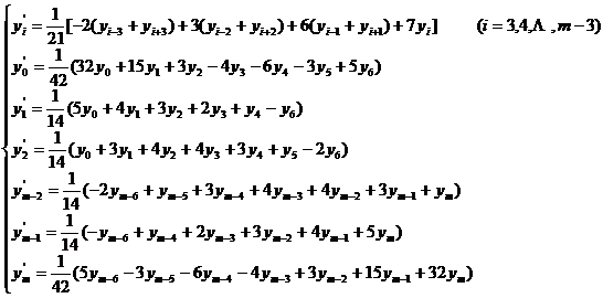
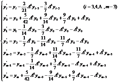
[ Take a seven-point moving average ] ( ie n = 3 )
or expressed by difference
4. Moving average method of cubic parabola
Following the notation of the second paragraph, the correction value is taken as the cubic parabolic equation![]()
![]()
![]() ( 2 )
( 2 )
The coefficients a, b, c, and d in the formula should be
![]() minimum
minimum
In the formula, t takes the 2 n +1 integer values closest to i in [0, m ] . When both are established, the coefficients a, b, c, d satisfy the following equations :![]()
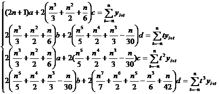
Solve a, b, c, d from this , and substitute it into ( 2 ) to get the corrected value .![]()
![]()
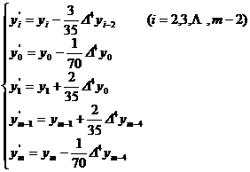
[ Take five-point moving average ] ( ie n = 2 )
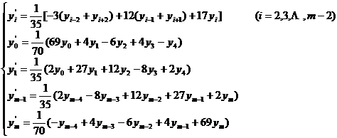
or expressed by difference
[ Take a seven-point moving average ] ( ie n = 3 )
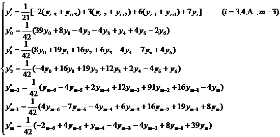
or expressed by difference
