§ 2 Multivariate function extreme value problem solution ( direct method )

 

This section discusses finding the objective function

Direct methods ( or experimental optimization methods ) for optimal solutions over defined regions , where

  ( represents the transpose of a vector )

Represents the column vector composed of the independent variables . Since the minimum and maximum are only the difference between the objective functions by one sign, only the dimension column vector is discussed here so that the

At this time, it is called the optimal solution ( optimal point ) .

[ Unimodal function ]   If the function has only one extreme point ( maximum point or minimum point ) on the region in question , then this function is called a multivariate unimodal function.

Multivariate unimodal functions can also be defined analytically. For example, let the function be defined on the area , since any route on the area can be used with a parametric equation

   

is represented, so the function along this route can also be represented with parameters as

    Assume                        

set again                            

if , when                   

, when

Then the function is said to be unimodal over the region from point to point , where

    Assume               

A function is said to be unimodal over a region if , for any pair of point sums on the region , there exists a route from passing to to over which the function is unimodal .

[ Factor Alternation Method ]   This method is to explore the optimal point in turn according to the direction of the coordinate axis . Set it as the unit vector of the i -th coordinate axis, that is

  

And given the allowable error in advance , the iterative procedure is as follows:

( 1 )   Select the initial point .

( 2 )   Starting from the initial point , firstly optimize along the direction of the first coordinate axis ( using the single factor method of § 1 ) to obtain a good point , namely

is a real parameter in the formula . Then the starting point is optimized along the direction of the second coordinate axis, and a good point is obtained , that is

And so on, until all directions are optimized, get , it satisfies

( 3 ) repeating step   ( 2 ) as a new initial point .

( 4 )   The above steps are carried out until starting from a certain initial point, no new point can be obtained after searching in all directions, or the distance from the previous initial point is less than the preset allowable error . This is the approximate solution of the optimal point .

[ Parallel line method ]  If one factor is difficult to adjust and another factor is easy to change in the two-factor problem being dealt with, it is inconvenient to use the two-factor alternation method, and the following parallel line method should be used instead:

Put the factors that are difficult to adjust on the vertical axis ( Figure 18.5) , and set the adjustable range as [ 0 , ] . Put the factors that are easy to change on the horizontal axis, and set the adjustable range as [ 0 , ]. The factor is fixed at the point , and on the straight line passing through this point and parallel to the horizontal axis, the factor is preferably on [ 0 , ] , and the good point is ① ; On the straight line , the pair factor is optimized on [ 0 , ] , and the good point is ② ; compare the quality of the two points ① and ② , if ② is better than ① , remove the upper half of the line ( if ① is better than 1)②Okay , just remove the lower half of the line ) , then fix the factor at the adjustable range, and select the factor on [ 0 , ] on the line passing through this point and parallel to the horizontal axis , and the good point is ③ ; Compare the quality of points ② and ③ . If ② is better than ③ , remove the lower half of the straight line and continue to narrow down the optimal range to find the approximate solution of the optimal point.

The selection of factors can also use the fractional method.

[ Blind Mountain Climbing Method ] The   iterative process is as follows:

(1)       Select the step size of the initial point ( base point ) , command .

(2)       Local exploration of the l -th direction ( ie, the axis direction ) of the k -th stage

where is the unit vector of the lth coordinate axis, first explore in the positive direction

V

If , then the exploration is successful, take this point as the starting point of the next exploration along the l +1th coordinate axis direction, and command ; otherwise, search in the opposite direction

If , the exploration is successful, take this point as the starting point of the next exploration along the l +1th coordinate axis direction, and order ;

and life .

When the local exploration along the directions of each coordinate axis is carried out in turn, the local exploration at this stage is also completed, and the best point of the kth stage is obtained at this time .

(3)       Command , consider the new base point, repeat step (2), if a better point cannot be obtained, reduce the step size and then perform local exploration until the step size is reduced to the specified accuracy, then the best point obtained is is the approximate solution of the optimal point.

Although the blind mountain climbing method ( also known as the exploratory mountain climbing method ) is not as fast as the previous methods, it is especially suitable for the situation where the factors cannot be greatly mobilized, or if a waste product is produced in large-scale production, it will cause a lot of losses.

[ Steep method and diagonal method ]

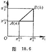
The 1 ° steepness and the steepness method are set at , two points have been tested, and their objective function values ​​are respectively ( Fig. 18.6) , and , then,   

      

is called the steepness from ascent to . There is a similar definition for dimensional space.

The objective function in the direction with large steepness obviously rises faster . The so-called steepness method is to use the obtained test results to calculate the steepness between points, and then take points in the direction with the greatest steepness ( favorable direction ) for testing. .

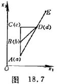2 ° Combined method ( the blind mountain climbing method is used in combination with the steepness method ). For example, the blind mountain climbing method is used to start from the point and move the factor along the axis to get the point . The effect is better, and the factor is still moved along the axis.   

The pixel gets a point ( Figure 18.7) , the effect is still good, and then along the axis

If the mobilization factor gets some points , the effect is good, and the next step is not necessarily from the

Hair and then along the vertical and horizontal direction to explore. At this time, the objective function can be calculated by

steepness of rise to , steepness of rise to , steepness of rise to

the steepness of , select a direction with the greatest steepness, for example , then

Next time, you can climb up in the direction of

Use the blind climbing method to climb up the extension line along the line section , or you can

The single-factor method is preferred, and a better point can generally be found .

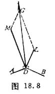3 ° Diagonal method Above , we compare the steepness of the three directions through the point to pick out a steeper direction, such as yes , but not   

It is not necessary to pass the steepest direction of the point, in fact, you only need to use the steepest direction of the two directions of the point.

degree, you can find the steeper direction of the point.

As shown in Figure 18.8 , take a point in the direction perpendicular to the

The length of is equal to the steepness of to, and and are on both sides of the

Take a point in the direction perpendicular to the

The steepness of , and and on both sides respectively , with , as the side

For a parallelogram, the direction of the diagonal is the point where the steepness is greatest

direction.

    [ Step acceleration method ] The step acceleration method is actually a combination of the blind mountain climbing method and acceleration in a favorable direction . The iterative procedure is as follows:

(1)      Select the initial point ( base point ) and step size , and order .

(2)      Blind mountain climbing ( see the blind mountain climbing method for the procedure ) .

    When the local exploration along the direction of each coordinate axis is carried out in turn, the local exploration at this stage is completed, and the next step can be accelerated in a favorable direction.

(3)      Speed ​​up hill climbing. life . If , then move to a new position to test for acceleration,

here

    Two situations may arise:

    1 ° If the value is improved, then , apply the method of step ( 2 ) to start a new exploration. 

    2 ° If the value of 2 ° does not improve, then cancel this acceleration and place the base point at the best point found last time, ie . command , start a new local exploration as in step (2) . 

    If it is found that the movement cannot be accelerated after a period , then reduce the step size and repeat step ( 2 ) . If successively reducing the step size can not accelerate the movement, this point is the approximate solution of the optimal point.

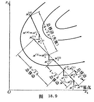
    The step-acceleration method is shown in Figure 18 in two dimensions . 9 shown.

    [ Direction acceleration method ( conjugate direction method )] The   iterative procedure is as follows:

    (1) Starting from the previous best numerical position ( which can be the point determined at the end of the previous iteration or a good point obtained by other methods ) and a set of linearly independent exploration directions ( which can take the direction of the coordinate axis ) . First find the best point on the straight line parallel to the passing point, and then find the best point on the straight line parallel to the passing point , and continue this process until all n exploration directions have been tried, and the final obtained point is . 

    (2) Find a special point , this point makes the value of the objective function improve the most compared with the previous point, that is, the point gives the maximum change of the movement , where . Also decide the vector . 

    (3) Calculation 

    (4) Remember if 

                                 ( 1 )

or

            ( 2 )

If that is not a good direction in the exploration, you should start the exploration again, starting from the last point and repeating step (1) in the same way, that is, and . If the inequalities (1), (2) are not satisfied, then explore along the direction until the minimum point is found. Define this point as , and the new exploration direction of stage k + 1 is ; ; and again . Then, starting from step (1) , the whole process is repeated until , where is a predetermined allowable error.

    Example of applying the directional acceleration method to find the objective function 

the minimum point.

    It is easy to find the absolute minimum point of the objective function by using the derivative method . Next, the directional acceleration method is used to find this minimum point. 

    Start exploring from the point , and use the sum to explore the direction .

    In the first stage , starting from the base point, one-dimensional exploration is carried out along the direction , and the moving distance is determined by 

Reaching a minimum, we get , therefore , while the objective function value is reduced by . Then explore in the same way along the direction , get , at the same time .

In order to decide whether to use the direction in the next stage, inequality (1) should be checked , the point is calculated , and , since , the direction is not used in the next stage .

The second stage The direction of this stage is the same as that of the previous stage ( because it is not adopted ) . One after another to explore , and , and . Recalculate points . Here , since , inequality (1) is not satisfied. Checking inequality (2) again , calculate 

where is the maximum change of the objective function in a given direction, ie . The right-hand side of inequality (2) is

Therefore, inequality (2) is not satisfied, that is, the direction can be adopted in the next stage

, explore along the direction to get the base point of the third stage as , and .

The third stage The exploration direction of this stage is sum . Exploring in these two directions will reveal that we cannot go any further, because in fact the absolute minimum has been found in the previous stage. Of course, this is not surprising since the objective function is quadratic. 

[ Direction step size double acceleration method ] The   iterative procedure is as follows:

Consider the kth stage

(1)         Select an initial point ( base point ) , a set of steps and a set of directions , where the upper index represents the first stage, and the lower index represents the first direction. At that time , the exploration direction was generally chosen to be parallel to the coordinate axis direction.

(2)         Perform successive explorations parallel to each of the n directions in turn. If the movement is successful, the new point is adopted, and if the movement is unsuccessful, the base point is retained. If the movement in a given direction is successful, the next time you explore in this direction, the step size will be doubled ; if it fails, it will be reduced to double , and the negative sign indicates exploration in the opposite direction. Generally take .

(3)         Until there is at least one success and one failure in each direction, the exploration along this direction ends. The last successful point is the new base point after the exploration in parallel to n directions is completed . The exploration direction of the next stage ( ie the first stage ) is calculated by the following equation:

First define the vector

where is the algebraic sum of all successful moves in the direction,

Then the direction is given by

in

In particular, where the main direction

Its components are

(4)         The above steps are carried out until ( for a predetermined allowable error ) , and the final base point obtained is approximately the optimal point.

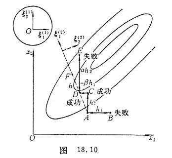
The directional step double acceleration method in two dimensions is shown in Figure 18.10 .

[ Simplex tuning method ] The   iterative procedure is as follows:

(1) Name the          n+ 1 vertices of the simplex of the n-dimensional space as , calculate the function value , compare the size, and determine

(2)         Find the symmetry point of the worst point

in the formula                          

(3)         If , it will be reduced to , defined by the following formula:

The requirement here is to avoid situations from happening.

If , then , and repeat the above steps.

If , then , and restart the iteration.

(4)         If , it will be expanded to , defined by the following formula:

The expanded condition can also be replaced by

or                      

If the above conditions are met, and

then                              

otherwise                              

and repeat the above steps.

The above process continues until

or                                

so far, where is a predetermined positive number.