§3
Differentiation
1. Differentiation of a function of one variable
1. Basic Concepts
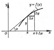
[ Definition of Derivative and Its Geometric Meaning ] Let the function y = f ( x ) when the independent variable has a change at the point x , the function y has a corresponding change , then when it tends to zero , the limit of the ratio exists ( a definite finite value ) , then this limit is called the derivative of the function f ( x ) at the point x , denoted as![]()
![]()
![]()
![]()
|
Figure 5.1 |
![]()
At this time, the function f ( x ) is said to be differentiable at point x ( or the function f ( x ) is differentiable at point x ) .
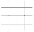
Geometrically , the derivative of the function f ( x ) is the slope of the tangent to the curve represented by the function y = f ( x ) at point x , i.e.![]()
![]() =
=![]()
where α is the angle between the tangent of the curve at point x and the x -axis ( Figure 5.1) .
[ one-sided derivative ]
![]() =
=![]()
![]()
and
![]() =
=![]()
![]()
are called the left and right derivatives of the function f ( x ) at point x , respectively.
The necessary and sufficient conditions for the existence of derivatives are :![]()
![]() =
=![]()
[ Infinite Derivative ] If at some point x there is
![]()
![]() = ±∞
= ±∞
Then the function f ( x ) is said to have infinite derivative at point x . At this time, the graph of the function y = f ( x ) is perpendicular to the x - axis at the tangent of the point x ( when =![]()
When + ∞ , the graph of the function f ( x ) is in the same direction as the y -axis at the positive tangent of the point x , and when = -∞ , the direction is opposite ) .![]()
[ The relationship between differentiability and continuity of functions ] If the function y = f ( x ) has a derivative at point x , then it must be continuous at point x . Conversely , continuous functions do not necessarily have derivatives , such as
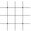
 The 1° function y = | x | is continuous at the point x = 0 , at the point x = 0, the left derivative = -1, the right derivative = 1, and the derivative does not exist ( Figure 5.2) .
![]()
![]()
![]()
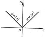 Figure 5.2 Figure 5.3 _
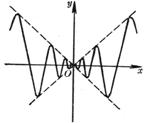
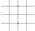
2° function
y = f ( x )=
Continuous at x = 0 , but no derivative exists around x = 0 ( Figure 5.3) .
2. The basic rules of taking derivatives
[ Four arithmetic derivation formulas ] If c is a constant , the function u = u ( x ) ![]() has derivatives , then
has derivatives , then
![]() =0
= c
=0
= c![]()
![]()
![]()
![]()
 ( ≠ 0 )
![]()
[ Derivative of composite function ] If y = f ( u ), u = both have derivatives , then![]()
![]() =
=![]()
[反函数的导数] 如果函数y=f(x)在点x有不等于零的导数,并且反函数x=f-1(y)在点y连续,那末![]() 存在并且等于
存在并且等于![]() ,即
,即
![]() =
=![]()
[隐函数的导数] 假定函数F(x,y)连续,并且对于每个自变量都有连续的偏导数,而且![]() ,则由
,则由
F(x,y)=0
所决定的函数y=f(x)的导数
![]() =
=![]() =
=![]()
式中![]() =
=![]() ,
,![]() =
=![]() (见本节,四)。
(见本节,四)。
[用参数表示的函数的导数] 设方程组
![]() (α<t<β)
(α<t<β)
式中![]() 和
和![]() 为可微分的函数,且
为可微分的函数,且![]() ,则由隐函数存在定理(本节,四,1)可把y确定为x的单值连续函数
,则由隐函数存在定理(本节,四,1)可把y确定为x的单值连续函数
y=![]()
而函数的导数可用公式
![]() =
=![]()
求得。
[用对数求导数法] 求一函数的导数,有时先取其对数较为便利,然后由这函数的对数求其导数。
例 求
![]()
的导数。
解 两边各取对数,得
lny=pln(x-a)+qln(x-b)-rln(x-c)
左边的lny为y的函数,而y又为x的函数,故应用求复合函数的导数的法则得到
![]()
由此得
![]()
所以
![]()
3.函数的微分与高阶导数
[函数的微分] 若函数y=f(x)的改变量可表为
![]() =A(x)dx+o(dx)
=A(x)dx+o(dx)
式中dx=Δx,则此改变量的线性主部A(x)dx称为函数y的微分,记作
dy=A(x)dx
函数y=f(x)的微分存在的充分必要条件是:函数存在有限的导数![]() =
=![]() ,这时函数的微分是
,这时函数的微分是
dy=![]() dx
dx
上式具有一阶微分的不变性,即当自变量x又是另一自变量t的函数时,上面的公式仍然成立.
[高阶导数] 函数y=f(x)的高阶导数由下列关系式逐次地定义出来(假设对应的运算都有意义):
![]() =
=![]()
![]()
[高阶微分] 函数y=f(x)的高阶微分由下列公式逐次定义:
![]() =
=![]()
![]()
式中![]() .并且有
.并且有
![]() =
=![]()
及
![]()
[莱布尼茨公式] 若函数u=![]() 及
及![]() =
=![]() 有n阶导数(可微分n次),则
有n阶导数(可微分n次),则
![]()
式中![]() ,
,![]() ,
,![]() 为二项式系数。
为二项式系数。
同样有
![]()
式中 ![]() ,
,![]()
更一般地有
式中m,n为正整数。
[ Higher-Order Derivatives of Composite Functions ] If the function y = f ( u ), u = has an l -order derivative, then![]()
in the formula
![]() ,
,![]()
[ Derivative table of basic functions ]
|
f ( x ) |
|
f ( x ) |
|
|
c |
0 |
|
|
|
x n |
nx n - 1 |
|
|
|
|
|
|
|
|
|
|
|
|
|
|
|
|
|
|
|
|
|
|
|
|
|
|
|
|
|
|
sh
x |
ch x |
|
|
|
ch
x |
sh x |
|
|
|
th
x |
|
|
|
|
cth
x |
|
|
|
|
sech
x |
|
|
|
|
csch
x |
|
|
|
|
|
|
|
|
|
Ar sech x |
f > 0 , take + |
|
|
|
Ar csch x |
|
Arch x=
|
f > 0 take + , f < 0 |
|
|
Arth x =
( |x|< 1) |
|
ln ch x |
th
x |
|
Arcth x=
( |x|>1) |
|
ln |
|


[ Table of Higher Derivatives of Simple Functions ]
|
f ( x ) |
|
|
|
m ( m - 1) … ( m - n +1) ( |
|
|
Here (2 n +1)!!=(2 n +1)(2 n - 1) |
|
|
|
|
|
|
|
|
|
|
|
|
|
|
|
|
|
|
|
|
|
|
|
|
|
|
|
|
sh x |
sh x ( n is even ) , ch x ( n is odd ) |
|
ch x |
ch x ( n is even ) , sh x ( n is odd ) |
4. Numerical derivatives
When a function is given in a graph or table , it is impossible to find its derivative by definition , only numerical derivatives can be found by approximation .
[ Graphical differentiation method ] is suitable for obtaining derivatives of functions given by graphics , such as known s - t diagrams , seeking diagrams , a - t diagrams, etc. in mechanical design. The basic steps are as follows:![]()
(1) Translate the original coordinate system Oxy along the negative direction of the y -axis by a distance to obtain the coordinate system ( Figure 5.4).![]()
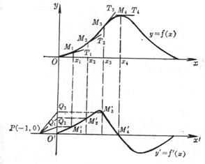
Figure 5.4
(2) Make a tangent M 1 T 1 through the point M 1 ( x 1 , y 1 ) on the curve y = f ( x ) and make a tangent M 1 T 1 . In the coordinate system , pass the point P ( -1,0) as PQ 1 parallel to M 1 T 1 intersects the y - axis at point Q 1 , then the ordinate of the point Q 1 ( point ) is the derivative . Take the ordinate of Q 1 as the ordinate![]()
![]()
![]() , x 1 is the abscissa to make a point .
, x 1 is the abscissa to make a point .![]()
(3) Take several points M 1 , M 2 , , on the curve y = f ( x ) , and obtain more dense points at the places where the curve is more curved . By imitating the above method , the corresponding points , , , and , are obtained in the coordinate system . Sub-connected into a smooth curve , that is, the graph of the derivative function .![]()
![]()
![]()
![]()
![]()
![]()
[ Difference quotient formula ] The following simple approximate formula is often used in practice
![]() , ,…,
, ,…,![]()
![]()
in the formula
![]() = ( 1st order difference of function f ( x ) at point a )
= ( 1st order difference of function f ( x ) at point a )![]()
![]() ( 2nd order difference of function f ( x ) at point a )
( 2nd order difference of function f ( x ) at point a )
………………………………
![]() ( k -th order difference of function f ( x ) at point a )
( k -th order difference of function f ( x ) at point a )
In the numerical table of the function , if there is an error , the deviation of the higher-order difference is large , so it is not appropriate to use the above formula to calculate the higher-order derivative .
[ Determining Numerical Derivatives Using Interpolation Polynomials ] Assuming that the interpolation polynomial P n ( x ) of the function y = f ( x ) has been found , it can be derived , then by approximation , given by![]()
![]()
f ( x )= P n ( x )+ R n ( x )
Omit the remainder , get
![]() ≈ ≈
≈ ≈![]()
![]()
![]()
and so on . Their remainders are correspondingly , , and so on .![]()
![]()
It should be noted that when the interpolating polynomial Pn ( x ) converges to f ( x ) , it does not necessarily converge to f ' ( x ) . Also , as h shrinks , the truncation error decreases , but the rounding error increases , so , The method of reducing the step size may not necessarily achieve the purpose of improving the accuracy . Due to the unreliability of using the interpolation method to calculate the numerical differentiation , during the calculation , special attention should be paid to the error analysis , or other methods should be used .![]()
[ Lagrange formula ] ( derived from Lagrangian interpolation formula , see Chapter 17 , §2, 3 )
![]()
in the formula 
![]()
![]()
![]() ( )
( )![]()
[ Markov formula ] ( derived from Newton's interpolation formula , see Chapter 17 , §2, 2 )
![]()
![]() ( )
( )![]()
In particular , when t = 0 , we have
![]()
![]()
![]()
![]()
![]()
[ Isometric formula ]
three point formula
![]() ≈
≈![]()
Four point formula
![]() ≈
≈![]()
Five point formula
![]() ≈
≈![]()
![]()
[ Using Cubic Spline Function to Calculate Numerical Derivative ] This method can avoid the unreliability of using interpolation method to calculate numerical derivative . Chapter 17 , §2, 4 ), when the interpolated function f ( x ) has a fourth-order continuous derivative , and hi = x i +1 - x i → 0 , as long as S ( x ) converges to f ( x ) ), then the derivative![]() must converge to , and S ( x ) - f ( x ) = O ( H 4 ) , - = O ( H 3 ), , where H is the maximum value of hi , therefore , the cubic spline function can be directly passed
must converge to , and S ( x ) - f ( x ) = O ( H 4 ) , - = O ( H 3 ), , where H is the maximum value of hi , therefore , the cubic spline function can be directly passed![]()
![]()
![]()
![]()
![]()
![]()
Find the numerical derivative
![]() =
=![]()
![]()
![]()
![]()
![]()
![]()
![]()
![]()
In the formula , , ( i =0,1,2, ) . ![]()
![]()
![]()
![]()
If only the derivative at the sample point x i is obtained , then
![]()
![]() ≈ =
≈ =![]()
![]()
![]() ≈ =
≈ =![]()
![]()
2. Differentiation of Multivariable Functions
[ Partial Derivatives and Their Geometric Meaning ] Let the binary function
u = f ( x , y )
当变量x有一个改变量Δx而变量y保持不变时,得到一个改变量
Δu=f(x+Δx,y)-f(x,y)
如果当Δx→0时,极限
![]()
![]() =
=![]()
![]()
存在,那末这个极限称为函数u=f(x,y)关于变量x的偏导数,记作![]() 或
或![]() ,也记作
,也记作![]() 或
或![]() ,即
,即
![]() =
=![]() =
=![]() =
=![]() =
=![]()
![]() =
=![]()
![]()
类似地,可以定义二元函数u=f(x,y)关于变量y的偏导数为
![]() =
=![]() =
=![]() =
=![]() =
=![]()
![]() =
=![]()
![]()
偏导数可以按照单变量函数的微分法则求出,只须对所论变量求导数,其余变量都看作常数.
偏导数的几何意义如下:
二元函数u=f(x,y)表示一曲面,通过曲面上一点M(x,y,u)作一平行于Oxu平面的平面,与曲面有一条交线,![]() 就是这条曲线在该点的切线与x轴正向夹角
就是这条曲线在该点的切线与x轴正向夹角![]() 的正切,即
的正切,即![]() =
=![]() .同样,有
.同样,有![]() =
=![]() (图5.5).
(图5.5).
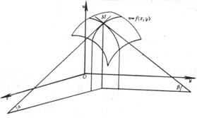
图5.5
偏导数的定义不难推广到多变量函数u=f(x1,x2,…,xn)的情形.
[偏微分] 多变量函数u=f(x1,x2,…,xn)对其中一个变量(例如x1 )的偏微分为
![]()
也可记作![]() .
.
[可微函数与全微分] 若函数u=f(x,y)的全改变量可写为
![]() =
=![]() +
+![]()
式中A,B与Δx,Δy无关,![]() ,则称函数u=f(x,y)在点(x,y)可微分(或可微),这时函数u=f(x,y)的偏导数
,则称函数u=f(x,y)在点(x,y)可微分(或可微),这时函数u=f(x,y)的偏导数![]() ,
,![]() 一定存在,而且
一定存在,而且
![]() =A,
=A, ![]() =B
=B
改变量Δu的线性主部
![]() =
=![]()
![]() +
+![]() dy
dy
称为函数u=f(x,y)的全微分,记作
du=![]()
![]() +
+![]() dy (1)
dy (1)
函数在一点可微的充分条件:如果在点(x,y)函数u=f(x,y)的偏导数![]() 存在而且连续,那末函数在该点是可微的.
存在而且连续,那末函数在该点是可微的.
公式(1)具有一阶微分的不变性,即当自变量x,y又是另外两个自变量t,s的函数时,上面的公式仍然成立.
上述结果不难推广到多变量函数u=f(x1,x2,…,xn)的情形.
注意,在一个已知点,偏导数的存在一般说来还不能确定微分的存在.
[复合函数的微分法与全导数]
1° 设u=f(x,y),x=![]() (t,s),y=
(t,s),y=![]() (t,s),则
(t,s),则
![]() =
=![]()
![]() +
+![]()
![]()
![]() =
=![]()
![]() +
+![]()
![]()
2° Let u = f ( x 1 , x 2 ,…, x n ), and x 1 , x 2 ,…, x n are all functions of t 1 , t 2 ,…, t m , then
![]()
![]()
……………………………………
![]()
3° Let u = f ( x , y , z ), and y = ( x , t ), z = ( x , t ), then![]()
![]()
![]() =
=![]()
![]()
![]() =
=![]()
4° Set u = f ( x 1 , x 2 ,…, x n ), x 1 = x 1 ( t ), x 2 = x 2 ( t ), , ![]() then the function u = f ( x 1 , x 2 , )
then the function u = f ( x 1 , x 2 , ) ![]() , the total derivative of
, the total derivative of
![]()
[ Homogeneous function and Euler's formula ] If the function f ( x , y , z ) satisfies the following relation identically
f ( tx , ty , tz )= f ( x , y , z )![]()
Then f ( x , y , z ) is said to be a homogeneous function of degree k . For this kind of function , as long as it is differentiable , we have
![]() ( Eulerian formula )
( Eulerian formula )
Note that the degree k of a homogeneous function can be any real number , for example , the function
![]()
It is a π -order homogeneous function of the independent variables x and y .
[ Differentiation of Implicit Functions ] Let F ( x 1 , x 2 ,…, x n , u )=0, then
……………………
![]()
( Refer to this section , IV ).
[ Higher-Order Partial Derivatives and Mixed Partial Derivatives ] The second-order partial derivatives of the function u = f ( x 1 , x 2 ,…, x n ) are , ,…, and , , ,…, the latter is called mixed partial derivatives . The third-order partial derivatives are , ,…, , , ,… . Higher-order partial derivatives can be defined similarly .![]()
![]()
![]()
![]()
![]()
![]()
![]()
![]()
![]()
![]()
![]()
The mixed partial derivative of the product of functions has the following formula : Let u be a function of ![]() x 1 , x 2 ,..., x n , then
x 1 , x 2 ,..., x n , then
Note that mixed partial derivatives are generally related to the order of derivation , but if two partial derivatives of the same order differ only in the order of derivation , then as long as the two partial derivatives are continuous , they must be equal to each other . For example , if At a certain point ( x , y ) the function and both are continuous , then there must be![]()
![]()
![]() ( x , y )= ( x , y )
( x , y )= ( x , y )![]()
[ Higher-Order Total Differentiation ] The second-order total differential of a binary function u = f ( x , y ) is
d 2 u =d(d u )=![]()
or abbreviated as
d 2 u =
The partial derivative symbols in the formula appear after squaring , , , and they act on the function u = f ( x , y ) , and the following are similar .![]()
![]()
![]()
![]()
![]()
The nth -order total differential of the binary function u = f ( x , y ) is
d n u =
The nth -order total differential of a multivariable function u = f ( x 1 , x 2 ,…, x m ) is
d n u =
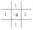
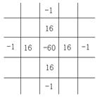
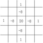
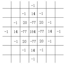
[ Differential Form of Partial Derivatives ]
( in the table h is the step size in the x -axis direction , and l is the step size in the y -axis direction )
|
icon |
Difference formula |
|||||||
|
|
|
|
||||||
|
|
|
|||||||
|
|
|
|
||||||
|
|
|
|||||||
|
|
|
|
||||||
|
|
|
|||||||
|
icon |
Difference formula |
|||||||
|
|
|
|
||||||
|
|
|
|||||||
|
|
|
|||||||
|
|
|
|
||||||
|
|
|
|||||||
|
|
|
|||||||
|
|
|
|
||||||
|
|
icon |
Difference formula |
||||||
|
|
|
|
||||||
|
|
|
|
||||||
|
|
|
|||||||
|
|
|
|||||||
|
|
|
|||||||
|
|
|
|||||||

3. Function determinant ( or Jacobian ) and its properties
n functions with n arguments
 (1)
(1)
They are defined in an n -dimensional region D , and have continuous partial derivatives with respect to the independent variable , then the determinant composed of these partial derivatives
It is called the functional determinant or Jacobian of function group (1) . Referred to as
![]()
Determinants of functions have a series of properties similar to ordinary derivatives .
1° In addition to the function group (1) , take the function group defined in the region P and having continuous partial derivatives
Assuming that when the point ( t 1 , t 2 , ) ![]() changes in P , the corresponding point ( x 1 , x 2 , ) does not go beyond the area D , then you can pass x 1 , x 2 ,
y 1 , y 2 , regarded as a composite function of t 1 , t 2 . At this time, we have
changes in P , the corresponding point ( x 1 , x 2 , ) does not go beyond the area D , then you can pass x 1 , x 2 ,
y 1 , y 2 , regarded as a composite function of t 1 , t 2 . At this time, we have![]()
![]()
![]()
![]()
![]()
![]() = (2)
= (2)![]()
It is the differential law for compound functions of one variable
y = f ( x ), x = ; =![]()
![]()
![]()
![]()
promotion.
2° In particular , if t 1 = y 1 , t 2 = y 2 , = y n (in ![]() other words , from the new variables x 1 , x 2 ,
other words , from the new variables x 1 , x 2 , ![]() and back to the old variables y 1 , y 2 , ),
and back to the old variables y 1 , y 2 , ), ![]() then It can be obtained by formula (2)
then It can be obtained by formula (2)
![]()
![]() =1
=1
It is the inverse function differentiation rule for unary functions
y = f ( x ), x = =![]()
![]()
![]()
promotion.
3° There are m ( m < n ) functions y 1 , y 2 , with n independent variables x 1 , x 2 , ![]() :
:![]()
where x 1 , x 2 are ![]() functions of m independent variables t 1 , t 2 :
functions of m independent variables t 1 , t 2 :![]()
Assuming that they all have continuous partial derivatives, then y 1 , y 2 , ![]() as functions of t 1 , t 2 ,
as functions of t 1 , t 2 , ![]() the expression of the functional determinant is
the expression of the functional determinant is
![]() =
=![]()
![]()
The sum on the right-hand side of the equation is taken from all possible combinations of n labels taken m at a time.![]()
When m = 1 , the above formula is the differential formula of the ordinary composite function
![]()
Generalization of . Especially when n = 3, m = 2 , there are
![]()
4° A system of equations consisting of n equations with 2 n independent variables
F i ( x 1 , x 2 , ; y 1 , y 2 , )=0 ( i =1,2,…, n )![]()
![]()
assumed
![]() ≠ 0
≠ 0
Consider y 1 , y 2 , as ![]() functions of x 1 , x 2 , determined by this equation system , then we have
functions of x 1 , x 2 , determined by this equation system , then we have![]()
![]()
It is the derivative formula of the implicit function y = f ( x ) determined by F ( x , y )=0
![]()
promotion .
The determinant of the 5° function can be used as a scaling factor for the area ( volume ) .
assumed function
u = u ( x , y ), = ( x , y )![]()
![]()
It is continuous on a certain region of the xy plane and has continuous partial derivatives , and it is assumed that on this region
![]() ≠ 0
≠ 0
Then d u d = d x d y
![]()
![]()
There are similar expressions for higher dimensional spaces .
Example of the transformation between Cartesian coordinates and spherical coordinates
x = r sin cos , y = r sin sin , z = r cos![]()
![]()
![]()
![]()
![]()
The determinant of the function is
![]() = =
= =
![]()
Then d x d y d z = d r d d = d r d d![]()
![]()
![]()
![]()
![]()
![]()