Four

4. Implicit function

1. Single variable implicit function

For by the equation

F ( x , y )=0

The determined implicit function has the following theorem :

[ Existence Theorem ] Let the function F ( x , y ) be defined in a certain neighborhood * R of the point M ₀ ( x ₀ , y ₀ ) and satisfy the following conditions :

(i) F ( x , y ) and its partial derivatives are continuous in R ,

(ii) F ( x ₀ , y ₀ )=0,

(iii) ≠ 0,

Then in some neighborhood of point M ₀ ( x ₀ , y ₀ )

; )

There is a unique single-valued function y = f ( x ) in it , which has the following properties :

1° F [ x , f ( x )] ≡ 0, and f ( x ₀ ) = y ₀ ,

2° The function f ( x ) is continuous in the interval ( ) ,

3° It has continuous derivatives in this interval .

[ Calculation of Derivatives ]

( ≠ 0)

2. Multivariate implicit function

For by the equation

F ( x , y , z )=0

The determined implicit function has the following theorem :

[ Existence Theorem ] Let the function F ( x , y , z ) be defined in a certain neighborhood R of the point P ₀ ( x ₀ , y ₀ , z ₀ ) and satisfy the following conditions :

(i) F ( x , y , z ) and its partial derivatives , continuous in R ,

(ii) F ( x ₀ , y ₀ , z ₀ )=0,

(iii) ( x ₀ , y ₀ , z ₀ ) ≠ 0,

Then in some neighborhood of point P ₀ ( x ₀ , y ₀ , z ₀ )

; ; )

There exists a unique single-valued function z = h ( x , y ) with the following properties :

1° F [ x , y , h ( x , y )] ≡ 0, and h ( x ₀ , y ₀ ) = z ₀ ,

The 2° function h ( x , y ) is continuous ,

3° It has continuous partial derivatives .

[ Calculation of Derivatives ]

, ( ≠ 0)

If you need to find all the first , second , and partial derivatives of each order , just replace the identity

F ( x , y , z )=0

Find the first - order , second ^- order , third - order ... _ _ _ _ _

Note that for the equation

F ( x ₁ , , x _n , y )=0

The identified implicit functions have similar results .

3. Implicit function determined by the system of equations

pair by the system of equations

(1)

The determined implicit function has the following theorem :

[ Existence Theorem ] Let the functions F ( x , y , z ) and G ( x , y , z ) be defined in a certain neighborhood R of the point P 0 ( _x 0 , _y 0 , _z 0 ) _and satisfy the following conditions :

(i) F ( x , y , z ), G ( x , y , z ) and all their partial derivatives are continuous in R ,

(ii) F ( x ₀ , y ₀ , z ₀ )=0, G ( x ₀ , y ₀ , z ₀ )=0,

(iii) Determinant

J ( x , y , z )=

At point P ₀ ( x ₀ , y ₀ , z ₀ ) is not equal to zero : J ( x ₀ , y ₀ , z ₀ ) ≠ 0.

Then in some neighborhood of point P ₀ ( x ₀ , y ₀ , z ₀ )

; ; )

There is a unique set of single-valued functions y = f ( x ), z = g ( x ) in , with the following properties :

1° F [ x , f ( x ), g ( x )] ≡ 0, G [ x , f ( x ), g ( x )] ≡ 0, and f ( x ₀ ) = y ₀ , g ( x ₀ )= z ₀ ,

2° In the interval ( ) , the functions f ( x ), g ( x ) are continuous ,

3° has continuous derivatives in this interval .

[ Calculation of Derivatives ] Consider y and z as implicit functions of x , and differentiate equation system (1) with respect to x to get

This is a system of linear equations with respect to and whose determinant J ≠ 0, from which and can be solved .

Note that for the system of equations

The identified implicit functions have similar results .

5. Variable Substitution in Differential Expressions

1. Univariate function

Let y = f ( x ), and have an expression containing the independent variable, the dependent variable, and their derivatives

H = F ( x , y , )

When used as variable substitution , each derivative can be calculated as follows:

[ In the case of independent variable transformation ] Let the transformation formula be

x =

At this time ,

(1)

………………

[ The case where both the independent variable and the function are transformed ] Let the transformation formula be

x = , y =

where t is the new independent variable and u is the new function .

At this time , by the differential law of the composite function, we get

……………………

Substitute these formulas into formula (1) to get the result .

2. Multivariate functions

[ In the case of independent variable transformation ] Let z = f ( x , y ), and there is an expression containing independent variables, dependent variables and their partial derivatives

H = F ( x , y , z , , , ,…)

The transformation formula is

x = , y =

where u and sum are new independent variables , then the partial derivative is determined by the following equation :

= +

Other higher-order partial derivatives can also be calculated in this way .

[ The case where both the independent variable and the function are transformed ] Let the transformation formula be

x = , y = , z =

where u , is the new independent variable , w = w ( u , v ) is the new function , then the partial derivative is determined by the following equation :

+ )+ + )= +

Other higher-order partial derivatives can also be calculated in this way .

Note that when H is not an individual partial derivative , but all the partial derivatives of the given order , it is more convenient to use the total differential when calculating the successive partial derivatives .

6. The Fundamental Theorem of Differential Calculus ( Mean Value Theorem )

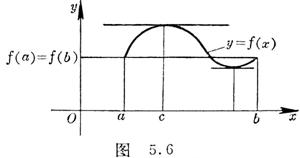
[ Lore's Theorem ] If (i) the function f ( x ) is defined on the closed interval [ a , b ] and is continuous , (ii) there is a finite derivative in the open interval ( a , b ) , and (iii) there is a finite derivative in the interval ( a , b ) The function values are equal at both ends of : f ( a ) = f ( b ). Then there is at least a point c between a and b , so that =0. That is, the curve y = f ( x ) is at point ( c , The tangent at f ( c )) is horizontal ( Fig. 5.6).

In particular , if f ( a ) = f ( b ) = 0, Lohr's theorem can be formulated as follows : between two roots of a function , its first derivative has at least one root .

Note that the function f ( x ) must be continuous on the closed interval [ a , b ] , and there must be a derivative in the open interval ( a , b ) , which is very important for the correctness of the conclusion of the theorem . For example, the function

f ( x ) = On the interval [0, 1] , all conditions of the theorem are satisfied except for the discontinuity when x = 1 , but = 1 everywhere in (0, 1) . For example, by the equation f ( The function defined by x ) = x ( ) and f ( x ) = ( ) also satisfies all the conditions of the theorem except when x = the ( bilateral ) derivative does not exist in this interval , but the derivative is in the left half It is equal to +1 in the interval and equal to +1 in the right half of the interval .

The condition (iii) of the theorem is also very important , for example, the function f ( x )= x on the interval [0,1] satisfies all the conditions of the theorem except condition (iii) , and its derivative is everywhere = 1.

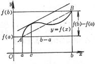
[ Mean Value Theorem ] If (i) f ( x ) is defined on the closed interval [ a , b ] and is continuous, and (ii) there is a finite derivative in the open interval ( a , b ) , then between a and b There is at least one point c between them , which satisfies the equation

= ( a < c < b ) (1)

Figure 5.7

That is, the tangent of the curve y = f ( x ) at the point ( c , f ( c )) is parallel to the chord AB ( Figure 5.7). This theorem is also known as the finite change theorem or Lagrange's theorem .

(1) is also often written in the following forms :

f ( b )

f ( x + Δ x ) Δ x ( x < c < x + Δ x )

Δ y = f ( x + Δ x ) ( )

From the mean value theorem we get

Theorem If every point on the interval [ a , b ] has =0, then the function f ( x ) is a constant on this interval .

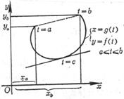
[ Cauchy's theorem ] If (i) the functions f ( t ) and g ( t ) are continuous in the closed interval [ a , b ] , (ii) have finite derivatives in the open interval ( a , b ) , and (iii) are in the open interval ( a , b ) In the interval ( a , b ) ≠ 0. Then there is at least a point c between a and b such that

Figure 5.8

= ( a < c < b )

This formula is called Cauchy's formula ( Figure 5.8). Cauchy's theorem is often called the generalized mean value theorem of differential calculus , since when g ( t ) = x , this formula is formula (1).

[ Mean Value Theorem for Multivariable Functions ] If (i) the function f ( x , y ) is defined over a closed region and is continuous , (ii) there are continuous partial derivatives inside this region ( ie, at all its interior points ) , , now examine two points in D

M ₀ ( x ₀ , y ₀ ) and M ₁ ( x ₀ + Δ x , y ₀ + Δ y )

Assuming that these two points can be connected by straight line segments M ₀M _{1 all located in the}D area , the following formula holds :

Δ f ( x ₀ , y ₀ ) = f ( x ₀ + Δ x , y ₀ + Δ y )

= (0< θ < 1)

From the mean value theorem we get

Theorem If the continuous function f ( x , y ) in the closed connected region D* , the partial derivatives in this region are all equal to zero , that is

= =0,

Then this function must be constant in region D.

7. Taylor formula and Taylor series

1. Taylor's formula for univariate functions

[ Taylor's local formula ] If the function f ( x ) satisfies the conditions : (i) it is defined in a certain neighborhood of point a , (ii) has a derivative up to order in this neighborhood , , (iii) has at point a The n -order derivative , then f ( x ) can be expressed in the following forms in the neighborhood of point a :

1° f ( a + h )= f ( a )+

* If any two points in the area can be connected by a "polyline", and all the points of the polyline are in this area, this area is called a connected area .

= ( as h → 0)

2° f ( x )= f ( a )+

= ( when x → a )

In particular , when a = 0 , there are

[ Maclaurin formula ]

f ( x )= f (0)+

= ( as x → 0)

[ Taylor formula ] If the function f ( x ) satisfies the conditions : (i) defined on the closed interval [ a , b ] , (ii) there is a continuous derivative up to the nth order on this closed interval , (iii) when a < There is a finite derivative when x < b , then f ( x ) can be expressed in the following forms on the closed interval [ a , b ] :

1° f ( a + h )= ( a < a + h < b )

where R _n ( h ) = (0 < θ < 1) ( Lagrange remainder )

or R _n ( h ) = (0 < θ < 1) ( Cauchy-type remainder )

2° f ( x )= ( )

where R _n ( x ) = ( a < ξ < b ) ( Lagrangian remainder )

or R _n ( x ) = (0 < θ < 1) ( Cauchy-type remainder )

In particular , when a = 0 , there are

[ Maclaurin formula ]

f ( x )= ( )

where R _n ( x ) = ( a < ξ < b ) ( Lagrangian remainder )

or R _n ( x ) = (0 < θ < 1) ( Cauchy-type remainder )

[ Taylor series ] In Taylor's formula 2° with remainder , if the expansion is raised to an arbitrarily high power of ( ) , we have

f ( x )= f ( a )+

Whether it converges or not , and whether its sum equals f ( x ), is called the Taylor series of the function f ( x ) . The coefficients of the power of ( )

f ( a ), , ,…, ,…

called the Taylor coefficient .

[ Maclaurin series ] In the Maclaurin formula with remainder , if the expansion proceeds to an arbitrarily high power of x , we have

f ( x )= f (0)+

Whether it converges or not , and whether its sum equals f ( x ), is called the Maclaurin series of the function f ( x ) . Coefficients of powers of x

f (0), , ,…, ,…

called the Maclaurin coefficient .

For the Taylor formula of polynomials ( Qin Jiushao's method ), see Chapter 3 , §2, 1 .

2. Taylor's formula for multivariate functions

[ Taylor formula ] Assume that the binary function f ( x , y ) in the neighborhood D of a certain point ( x ₀ , y ₀ ) has all continuous partial derivatives up to the n +1 order . Give x and y a change h and k , so that the straight line segment connecting the points ( x ₀ , y ₀ ) and ( x ₀ + h , y ₀ + k ) does not go beyond D ,Then f ( x , y ) can be expressed in D in the form :

1° f ( x ₀ + h , y ₀ + k )=

(0< θ < 1)

The symbol in the formula

The meaning is as follows : treat , as a number ( rather than as a symbol for differential operations ), and expand it according to the binomial formula , we get

= =

2 ⁰

In particular , when x ₀ =0, y ₀ =0 , we get

[ Maclaurin formula ]

f ( x , y )=

Similar formulas exist for multivariate functions of more than two variables .

[ Taylor series ] In the above Taylor formula 2° , if the expansion is carried out to any high power of ( ) and ( ) , there are

f ( x , y )=

Regardless of whether it converges or not , and whether its sum equals f ( x , y ), it is called a Taylor series of f ( x , y ) .

[ Maclaurin series ] In the above Maclaurin formula , if the expansion is carried out to any high power of x , y , there is

f ( x , y )= f (0,0)+

Whether it converges or not , and whether its sum equals f ( x , y ), it is called the Maclaurin series of f ( x , y ) .

Eight, power series

1 . single variable power series

[ definition ] a series of the following form

( 1 )

(where a ₀ , a ₁ , are real constants) is called the power series of x . More generally, the series

( where a is a real constant ) is also called a power series .

[ Absolutely convergent ] If the series ( 1 ) converges when x = , then the series ( 1 ) converges absolutely for any value of x satisfying | x | < || .

[ Convergence radius and convergence interval ] For any power series, there is a number R (0 ≤ R <+ ∞ ), so that when | x | < R , the series absolutely converges, when | x | > R , The series diverges . This number R is called the radius of convergence of a given series, the interval (-R, R ) is called its convergence interval, and at the two endpoints of the interval x = R and x = - R , the series may Convergence can also diverge .

The radius of convergence R can be calculated according to the Cauchy - Hadamard formula

or the formula R =

Compute ( if limit exists ).

[ Abel's theorem ] If the power series S ( x ) = ( | x |< R ) converges at the endpoint x = R of the convergence interval, then

S ( R )=

[ Internally closed uniform convergence ] If the radius of convergence of the series ( 1 ) is equal to R , then for any satisfying 0<< R , the series ( 1 ) converges uniformly on the interval [ , ] .

[ Continuous ] The sum of the power series is continuous at every point in the convergence interval .

[ itemwise integration ] At any point x within the convergence interval of the series ( 1 ) , there is

where S ( x ) represents the sum of series ( 1 ) .

[ itemwise differentiation ] The sum S ( x ) of a power series ( 1 ) is differentiable at any point within the convergence interval of this series .

has the same radius of convergence as ( 1 ), and the sum of this series is equal to .

[ Higher-Order Derivative ] If the series ( 1 ) has a radius of convergence R , then its sum S ( x ) has an arbitrary derivative at any point in the interval ( , R ) , and the function ( n =1, ) is The sum of the series (whose radius of convergence is also R ) obtained n times of the term differential order ( 1 )

= ( < x < R )

2 . Multivariate Power Series

[ Power series of two variables ] According to the positive integer powers of the variables x and y , the form is as follows

( 2 )

The heavy series is called the power series of bivariate x , y .

The study of the range of convergence of multivariate power series differs in many ways from univariate, but there are still

Theorem If the series ( 2 ) converges when x = x ₀ , y = y _{0 , then when}

| x |<| x ₀ |,| y |<| y ₀ |

, the series also converges .

[ Convergence range ] If M is a region of two variables x , y , where the power series ( 2 ) converges at each point, and diverges at the points outside it, it may be possible at the boundary points Divergence, it may also converge . Then the region M is called the convergence range of the power series ( 2 ) .

The convergence range of a bivariate power series is not necessarily of the form | x |< R ₁ , | y |< R ₂ , e.g.

1 ° series

The range of convergence is | x |<1 , | y |<1.

2° series

Condensed everywhere .

3° series

=1+ x + + xy + x ²y + x ³y + + x ²y ² +

( =(1+ x + )[1+ xy + ]= )

The range of convergence is | x |<1 , | xy |<1.

The above results are easy to generalize to multivariable power series .

3 . Power series expansion of a function

[ Uniqueness theorem of power series ] If the function f ( x ) ( or f ( x , y ) ) can be expanded into a power series at x = 0 ( or x = 0, y = 0)

f ( x )=

Then this power series is its Maclaurin series .

[ Existence Theorem of Power Series ]

1° if the function f ( x ) has any derivative at x = 0 and when ≤ x ≤ R

where R _n ( x ) is the remainder of the Maclaurin formula, then the function f ( x ) can be expanded into a power series in the interval ≤ x ≤ R. In fact, it can be proved that there is a function generated by the function f ( x ) Maclaurin series, although it converges, its sum is not equal to f ( x ).