Fourth, the method of definite integral
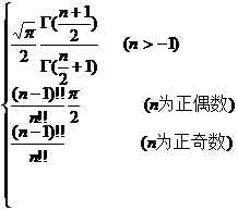
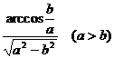
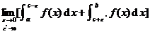
[ Properties of Definite Integrals ]
![]()
![]()
![]()
![]()
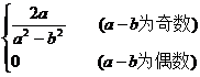
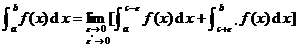
[ Integration by parts ]
![]()
in the formula![]()
[ Variable substitution method ] Assuming that the function has continuous derivatives in the interval [ ] , and the function is continuous in the interval , and changes monotonically from to , then![]()
![]()
![]()
![]()
![]()
![]()
![]()
![]()
![]()
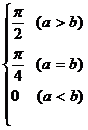
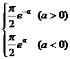
[Using function parity quadrature method] If it is an even function, then
![]()
![]()
If it is an odd function, then![]()
![]()
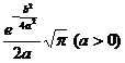
[Derivation of parameters by integral method] Suppose f ( x , t ) is continuous in the bounded region , and there are continuous partial derivatives , then at that time , there are![]()
![]()
![]()
![]()
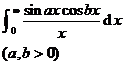
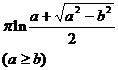
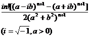
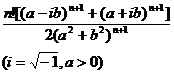
Example Calculating Integral![]()
De-assign![]()
Then . Because![]()
![]()
![]()
![]()
So︳ .![]()
[Definite integral table]
|
Definite integral |
Definite integral value |
|
|
|
|
|
|
|
|
|
|
Definite integral |
Definite integral value |
|
|
|
|
|
|
|
|
|
|
|
|
|
|
|
|
|
|
|
|
|
|
|
|
|
|
|
|
|
|
|
|
|
|
|
|
|
|
|
|
|
|
|
|
|
|
|
|
|
Definite integral |
Definite integral value |
|
|
|
|
|
|
|
|
|
|
|
|
|
|
|
|
|
|
|
|
|
|
|
|
|
|
|
|
|
|
|
|
|
|
|
|
|
|
|
|
|
|
|
|
|
|
|
|
|
|
|
|
|
|
|
|
|
|
Definite integral |
Definite integral value |
|
|
|
|
|
|
|
|
|
|
|
|
|
|
|
|
|
|
|
|
|
|
|
|
|
|
|
|
|
|
|
|
|
|
|
|
|
|
|
|
|
|
|
|
|
|
|
|
|
|
|
|
|
|
|
|
|
|
|
|
|
Definite integral |
Definite integral value |
|
|
|
|
|
|
|
|
|
|
|
|
|
|
|
|
|
|
|
|
|
|
|
|
|
|
|
|
|
|
|
|
|
|
|
|
|
|
|
|
|
|


5. Generalized integral
1. The concept of generalized integral
[Infinite finite generalized integral] Let the function f ( x ) be integrable on [ a , b ] , u > a , < b , u > , when the limit on the right side of the following equations exists, ![]()
![]()
![]()
![]()
![]()
In this case, the infinite generalized integral is called convergence, otherwise it is called divergence .
[ Generalized integral of unbounded functions ] Let the function f ( x ) have only one flaw point x = c on the given interval [ a , b ] , that is, the function f ( x ) is unbounded in the neighborhood of the point x = c, and in [ a , b ] a , c - ε ] and [ c + ε ', b ] are integrable, ε , ε ' are any small positive numbers, when ε and ε ' tend to zero independently, the limit
 (1)
(1)
If exists, then use the above formula to define the imperfect integral of the unbounded function f ( x ) from a to b , denoted as
[ Cauchy's principal value ] Sometimes the limit ( 1 ) does not exist, but if ε '= ε → 0 , this limit ( 1 ) exists, it is called the principal value of the integral , denoted as![]()
![]()
At this time, the generalized integral of unbounded function is said to converge in the sense of principal value, otherwise it is called divergence .
[ Absolute Convergence and Conditional Convergence ] If the generalized integral of f ( x ) and the generalized integral of | f ( x )| converge at the same time, then the generalized integral of f ( x ) is said to be absolutely convergent , and f ( x ) is called absolutely integrable ; if only the former converges and the latter does not, then the generalized integral of f ( x ) is said to be conditionally convergent .
2. Generalized integral convergence criterion
The necessary and sufficient condition for 1 ° convergence is: for any given ε > 0 , there exists N = N ( ε )>0, as long as there is | |< ε . ![]()
![]()
![]()
2 ° If f ( x ) is non-negative , the necessary and sufficient conditions for convergence are: ![]()
F ( u )=![]() is a bounded function.
is a bounded function.
3 ° When x →∞, f ( x ) = . If p > 1, it converges; if p ≤ 1, it diverges . ![]()
![]()
![]()
4 ° Convergence if g ( x ) is monotonically bounded ( x ≥ a ) . ![]()
![]()
5 ° Let f ( x ) ≥ 0, g ( x ) ≥ 0, and f ( x ) ≤ cg ( x ) ( x ≥ a , c is a constant greater than zero) . If it converges, it also converges; if it diverges , it also diverges . ![]()
![]()
![]()
![]()
6 ° The relationship between infinite series and generalized integral: Let f ( x ) be a positive non-increasing continuous function defined on the interval [ a , ∞ ) , then the series f ( a )+ f ( a +1)+ · · + f ( a + k )+ · · Convergence or divergence at the same time as the integral . ![]()
The necessary and sufficient conditions for the convergence of the 7 ° generalized integral (with a as the flaw point) are: for any given ε > 0 , there exists δ ( a < δ < b ), such that when a < u '< u ''< δ time | |< ε . ![]()
![]()
8 ° Let g ( x ) have continuous derivatives and be a constant positive, monotonically decreasing function, and if there is a constant M such that for all u > a , there is | |< M , then the generalized integral converges . ![]()
![]()
![]()
6. Integral with parameters
1. Regular integral with parameters
[ Continuity ] If the binary function f ( x , y ) is defined and continuous over the bounded region R ( a ≤ x ≤ A , b ≤ y ≤ B ) , then
![]()
is a continuous function on the closed interval [ b , B ] .
[ Differentiation under the integral sign ] If f ( x , y ) is continuous in the bounded region R ( a ≤ x ≤ A , b ≤ y ≤ B ) , and there is a continuous partial derivative (x, y) , then when b < y < B ,![]()
![]()
In general, when the integral limit is the sum of differentiable functions of parameters y , and when b ≤ y ≤ B , a ≤ ≤ A ,![]()
![]()
![]()
When a ≤ ≤ A ,![]()
![]() (1)
(1)
[ Derivative operation of integral ] The following formula is a special case of ( 1) .
![]()
![]()
![]()
![]()
![]()
[ Integration under the integral sign] If the function is continuous over the bounded region [ a ≤ x ≤ A , b ≤ y ≤ B ] , then![]()
![]()
2. Generalized integral with parameters
[ Consistent convergence ] Let the function f ( x , y ) be a continuous function defined in the region R ( a ≤ x < ∞ , y 1 < y < y 2 ) , if for any given ε > 0 , there exists A positive number B = B ( ε ) only related to ε , so that when b ≥ B , for all y inequalities in the interval ( y 1 , y 2 )
![]()
are all established, then the generalized integral is said to converge uniformly in the interval ( y 1 , y 2 ) , and it is a continuous function of the parameter y in this interval .![]()
[ Consistent Convergence Discrimination Method ]
1 ° Cauchy discriminant integral
![]()
The necessary and sufficient condition for uniform convergence in the interval ( y 1 , y 2 ) is: for any ε > 0 , there is a positive number B = B ( ε ), such that when b '> B , b ''> B , for All y in the interval ( y 1 , y 2 ) , have
![]()
2 ° Weyl-Strass discriminant Assuming that the function f ( x , y ) ( a function of x ) is integrable over any finite interval [ a , A ] , if there is a function F ( x ) that is independent of the parameter y , it integrable over the interval [ a , ∞ ) and for all y in the interval ( y 1 , y 2 )
| f ( x ,y )| ≤ F (x) ( x ≥ a )
then points
![]()
Converges uniformly in the interval ( y 1 , y 2 ) .
[ Differentiation with respect to parameters ] If (i) the function f ( x , y ) is continuous in the region R ( a ≤ x < ∞ , y 1 < y < y 2 ) and is differentiable with respect to the parameter y , (ii) the integral Convergence, (iii) the integral converges uniformly in the interval ( y 1 , y 2 ) , then when y 1 < y < y 2 ,![]()
![]()
![]()
[ Integration over parameters ] If the function f ( x , y ) is continuous in the region R ( a ≤ x < ∞ , y 1 < y < y 2 ) and converges uniformly in the interval ( y 1 , y 2 ) , but ![]()
![]()
7. Sturgess Points
[ Definition ] Suppose two bounded functions f ( x ) and g ( x ) are given on the interval [ a , b ] . Divide the interval [ a , b ] into several parts by any method , and the dividing points are
a = x 0 < x 1 < x 2 < … < x i < x i+ 1 < … < x n = b
And let λ be the largest of Δ x i = x i + 1 - x i ( t = 0,1 , . _![]()
![]()
σ =![]()
When λ → 0 , if a limit exists, then this limit is called the Sturgess integral of the function f ( x ) over the function g ( x ) , denoted by![]()
![]()
In particular, when the function g ( x ) is continuously differentiable over the interval, the Styrgis integral of the function f ( x ) with respect to g ( x ) is the usual Riemann integral
![]()
[ integrability ]
1 °If the function f ( x ) is continuous and the function g ( x ) has bounded variation, then the integral
![]() ( 1 )
( 1 )
exist .
2 °If the function f ( x ) is Riemann-integrable over the interval [ a , b ] , the function g ( x ) satisfies the Lipschitz condition:
| g ( x ') - g ( x '' )| ≤ L ( x ' - x '')
( L is a constant, a ≤ x ''< x ' ≤ b )
Then the integral (1) exists .
3 °If the function f ( x ) is Riemann-integrable over the interval [ a , b ] , the function g ( x ) can be expressed as
g ( x ) = C +![]()
where C is a constant, and the function is absolutely integrable on the interval [ a , b ] , then the integral (1) exists .![]()
[ Integration rule and inequalities ]
1 ° integration rule
![]()
![]()
![]()
![]() ( k , l are constants )
( k , l are constants )
![]()
( a < c < b , all three integrals exist . When the two integrals on the right side of the above formula exist, one
Generally, it is not possible to introduce the existence of points)![]()
![]() ( Integral by Parts formula )
( Integral by Parts formula )
2 ° If g ( x ) is a non-decreasing function on the interval [ a , b ] , then
![]() ≤
≤![]()
3 ° If g ( x ) is a non-decreasing function on the interval [ a , b ] , then f ( x ) ≤ F ( x ), then
![]() ≤
≤![]()
8. Approximate Calculation of Integral
1. Interpolation and quadrature formula
[ General formula for equidistant interpolation quadrature (Coster formula) ]
![]() ≈ ( b - a )
≈ ( b - a )![]()
where is the equidistant node:![]()
![]() = a + kh k =0 ,1,2 , … , n
= a + kh k =0 ,1,2 , … , n
![]()
![]() is the Cotes coefficient (see table below) .
is the Cotes coefficient (see table below) .
Cotes coefficient table
|
n |
|
0 |
|
1 |
|
2 |
|
3 |
|
4 |
|
5 |
|
6 |
|
7 |
|
8 |
|
9 |
|
10 |
|
1 |
|
|
|
|
|
|
|
|
|
|
|
|
|
|
|
|
|
|
|
|
|
|
|
2 |
|
|
|
|
|
|
|
|
|
|
|
|
|
|
|
|
|
|
|
|
|
|
|
3 |
|
|
|
|
|
|
|
|
|
|
|
|
|
|
|
|
|
|
|
|
|
|
|
4 |
|
|
|
|
|
|
|
|
|
|
|
|
|
|
|
|
|
|
|
|
|
|
|
5 |
|
|
|
|
|
|
|
|
|
|
|
|
|
|
|
|
|
|
|
|
|
|
|
6 |
|
|
|
|
|
|
|
|
|
|
|
|
|
|
|
|
|
|
|
|
|
|
|
7 |
|
|
|
|
|
|
|
|
|
|
|
|
|
|
|
|
|
|
|
|
|
|
|
8 |
|
|
|
|
|
|
|
|
|
|
|
|
|
|
|
|
|
|
|
|
|
|
|
9 |
|
|
|
|
|
|
|
|
|
|
|
|
|
|
|
|
|
|
|
|
|
|
|
10 |
|
|
|
|
|
|
|
|
|
|
|
|
|
|
|
|
|
|
|
|
|
|
When the interval [ a , b ] is smaller, the result given by the Cotes formula is more accurate . Therefore, when the interval [ a , b ] is larger, in order to avoid using the Cotes formula with a larger n value, it is often necessary to use [ a , b ] N equal parts, apply the Cotes formula with a smaller n value to each of the equal parts, and then add the integral values of each equal part to obtain the integral over the interval [ a , b ] values, such as the following trapezoid formula ( n = 1) and Simpson formula ( n = 2).
[ Trapezoid formula ]
![]() ≈
≈![]()
![]() = a + kh , k =1,2, … , N - 1
= a + kh , k =1,2, … , N - 1
![]()
If ≤ M 2 , the truncation error is![]()
![]() ≤
≤![]()
[ Simpson formula ]
![]() ≈
≈![]()
![]() = a + k
= a + k![]() ,
, ![]()
If ≤ , then the truncation error is![]()
![]()
![]() ≤
≤![]()
[ Loombe formula ] set
![]()
![]()
=![]()
![]()
but
![]()
![]()
In general, m can be appropriately selected to make it fixed, and then increase k to make the approximate truncation error
![]()
within the allowable error range, then
![]() ≈
≈![]()
The specific calculation process can be carried out from left to right and top to bottom according to the following table (the direction of the arrow in the table indicates the calculation sequence) .

Example Calculating Integral with Lombe's Formula
![]()
![]()
The error does not exceed 0.0000001.
Solution here , a =0, b =1. It can be calculated in five steps, and the results are as follows: ![]()
(1)
![]()
(2)
![]()
![]()
(3)
![]()
![]()
![]()
(4)
![]()
![]()
![]()
![]()
(5) can continue to calculate
![]() 3.140941614 3.141592655
3.140941614 3.141592655
![]()
![]() 3.141592665 3.141592643
3.141592665 3.141592643
![]()
because
| - |=|3.141592643 ![]()
![]() - 3.141592665|<0.0000001
- 3.141592665|<0.0000001
so
![]() ≈ 3.14159264
≈ 3.14159264
while the exact value is
![]()
![]()
Among the isometric interpolation and quadrature formulas, the Simpson formula and the Longbei formula are better, the calculation is simple , it is easy to realize on the electronic computer ( there are standard programs ) , and the accuracy is quite high . In particular, the Longbei formula uses interval successive The method of dividing in half , the function value obtained by the previous division can still be used after the interval is divided into half , which has the advantages of regular calculation and no need to store the Cotes coefficient and nodes .
But the equidistant interpolation quadrature formula cannot compute generalized integrals . Generalized integrals can only be computed using the following Gaussian quadrature formula .
[ Differential interpolation formula (Gaussian formula ) ]
The Gaussian quadrature formula is
![]() ≈ n =1,2, …
≈ n =1,2, …![]()
where the interval ( a , b ) can be finite or infinite, and w ( x ) is a non-negative weight function in the interval ( a , b ) .
-∞≤ a ≤ < < … < < b ≤∞![]()
![]()
![]()
is the quadrature node (the root of the corresponding orthogonal polynomial), ( k =1,2, … , n ) is the quadrature coefficient . When f ( x ) is a polynomial not exceeding 2 n - 1 degree, the above quadrature formula (1) becomes an equation .![]()
A few exceptions are listed below .
1 °![]()
( - 1 < θ < 1)
where is the roots of the Legendre polynomial ( see Chapter XII, § 2 , a) .![]()
![]()
2 °![]()
( - 1 < θ < 1)
where are the roots of Chebyshev polynomials of the first kind ( see Chapter XII, § 2 , 2) .![]()
![]()
It can also be expressed as
![]()
3 ° ![]()
( - 1 < θ < 1)
where are the roots of Chebyshev polynomials of the second kind ( see Chapter XII, § 2 , 3) .![]()
![]()
4 °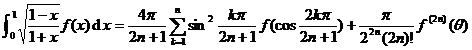
( - 1 < θ < 1)
5 °![]()
2.
The product node and the product coefficient table of the Gaussian product formula
[ Gaussian quadrature formula ]
![]()
where are the roots of the Legendre polynomial .![]()
![]()
|
n |
quadrature node |
Multiplying coefficient |
|
2 |
|
1 |
|
3 |
0
|
0.88888 88889 0.55555 55556 |
|
4 |
|
0.65214 51549 0.34785 48451 |
|
5 |
0
|
0.56888 88889 0.47862 86705 0.23692 68851 |
|
6 |
|
0.46791 39346 0.36076 15731 0.17132 44924 |
|
7 |
0
|
0.41795 91837 0.38183 00505 0.27970 53915 0.12948 49662 |
|
8 |
|
0.36268 37834 0.31370 66459 0.22238 10345 0.10122 85363 |
|
n |
quadrature node |
Multiplying coefficient |
|
9 |
0
|
0.33023 93550 0.31234 70770 0.26061 06964 0.18064 81607 0.08127 43884 |
|
10 |
|
0.29552 42247 0.26926 67193 0.21908 63625 0.14945 13492 0.06667 13443 |
[ Lebeteau quadrature formula ]
![]()
The root of the formula .![]()
![]()
|
n |
quadrature node |
Multiplying coefficient |
|
3 |
0 |
0.33333 333 1.33333 333 |
|
4 |
|
0.16666 667 0.83333 333 |
|
5 |
0 |
0.10000 000 0.54444 444 0.71111 111 |
|
6 |
|
0.06666 667 0.37847 496 0.55485 838 |
|
7 |
0 |
0.04761 904 0.27682 604 0.43174 538 0.48761 904 |
|
8 |
|
0.03571 428 0.21070 422 0.34112 270 0.41245 880 |
|
9 |
0 |
0.02777 77778 0.16549 53616 0.27453 87126 0.34642 85110 0.37151 92744 |
|
10 |
|
0.02222 22222 0.13330 59908 0.22488 93420 0.29204 26836 0.32753 97612 |
[ Laguerre's quadrature formula ]
![]()
![]()
where is the root of the Laguerre polynomial (see Chapter XII, § 2 , 4) .![]()
![]()
|
n |
quadrature node |
Multiplying coefficient |
|
|
2 |
0.58578 64376 3.41421 35624 |
(-1)8.53553 39059* (-1)1.46446 60941 |
1.53332 60331 4.45095 73351 |
|
3 |
0.41577 45568 2.29428 03603 6.28994 50829 |
(-1)7.11093 00993 (-1)2.78517 73357 (-1)1.03892 56502 |
1.07769 28593 2.76214 29619 5.60109 46254 |
|
4 |
0.32254 76896 1.74576 11012 4.53662 02969 9.39507 09123 |
(-1)6.03154 10434 (-1)3.57418 69244 (-2)3.88879 08515 (-4)5.39294 70556 |
0.83273 91238 2.04810 24385 3.63114 63058 6.48714 50844 |
|
5 |
0.26356 03197 1.41340 30591 3.59642 57710 7.08581 00059 12.64080 08443 |
(-1)5.21755 61058 (-1)3.98666 81108 (-2)7.59424 49582 (-3)3.61175 86799 (-5)2.33699 72386 |
0.67909 40422 1.63848 78736 2.76944 32424 4.31565 69009 7.21918 63544 |
|
6 |
0.22284 66042 1.18893 21017 2.99273 63261 5.77514 35691 9.8374674184 15.98287 39806 |
(-1) 4.58964 67395 (-1)4.17000 83077 (-1)1.13373 38207 (-2)1.03991 97453 (-4)2.61017 20282 (-7)8.98547 90643 |
0.57353 55074 1.36925 25907 2.26068 45934 3.35052 45824 4.88682 68002 7.84901 59456 |
|
7 |
0.19304 36766 1.02666 48953 2.56787 67450 4.90035 30845 8.18215 34446 12.73418 02918 19.39572 78623 |
(-1)4.09318 95170 (-1)4.21831 27786 (-1)1.47126 34866 (-2)2.06335 14469 (-3)1.07401 01433 (-5)1.58654 64349 (-8)3.17031 54790 |
0.49647 75975 1.17764 30609 1.91824 97817 2.77184 86362 3.84124 91225 5.38067 82079 8.40543 24868 |
|
8 |
0.17027 96323 0.90370 17768 2.25108 66299 4.26670 01703 7.04560 54024 10.75851 60102 15.74067 86413 22.86313 17369 |
(-1)3.69188 58934 (-1)4.18786 78081 (-1)1.75794 98664 (-2)3.33434 92261 (-3)2.79453 62352 (-5)9.07650 87734 (-7)8.48574 67163 (-9)1.04800 11749 |
0.43772 34105 1.03386 93477 1.66970 97657 2.37692 47018 3.20854 09134 4.26857 55108 5.81808 33687 8.90622 62153 |
|
9 |
0.15232 22277 0.80722 00227 2.00513 51556 3.78347 39733 6.20495 67779 9.37298 52517 13.46623 69111 18.83359 77890 26.37407 18909 |
(-1)3.36126 42180 (-1)4.11213 98042 (-1)1.99287 52537 (-2)4.74605 62766 (-3)5.59962 66108 (-4)3.05249 76709 (-6)6.59212 30261 (-8)4.11076 93304 (-11)3.29087 40304 |
0.39143 11243 0.92180 50285 1.48012 79099 2.08677 08076 2.77292 13897 3.59162 60681 4.64876 60021 6.21227 54198 9.36321 82377 |
* ![]() represents a number , other similarities, .
represents a number , other similarities, .![]()
![]()
[ Hermitian quadrature formula ]
![]()
![]()
where is the root of the Hermitian polynomial (see Chapter XII, § 2 , 5) .![]()
![]()
|
n |
quadrature node |
Multiplying coefficient |
|
|
2 |
|
(-1)8.86226 92545* |
1.46114 11827 |
|
3 |
0
|
(0)1.18163 59006 (-1)2.95408 97515 |
1.18163 59006 1.32393 11752 |
|
4 |
|
(-1)8.04914 09001 (-2)8.13128 35447 |
1.05996 44829 1.24022 58177 |
|
5 |
0
|
(-1)9.45308 72048 (-1)3.93619 32315 (-2)1.99532 42059 |
0.94530 87205 0.98658 09968 1.18148 86255 |
|
6 |
|
(-1)7.24629 59522 (-1)1.57067 32032 (-3)4.53000 99055 |
0.87640 13344 0.93558 05576 1.13690 83327 |
|
7 |
0
|
(-1)8.10264 61756 (-1)4.25607 25261 (-2)5.45155 82819 (-4)9.7178124510 |
0.81026 46176 0.82868 73033 0.89718 46002 1.10133 07296 |
|
8 |
|
(-1)6.61147 01256 (-1)2.07802 32582 (-2)1.70779 83007 (-4)1.99604 07221 |
0.76454 41287 0.79289 00484 0.86675 26066 1.07193 01443 |
|
9 |
0
|
(-1)7.20235 21561 (-1)4.32651 55900 (-2)8.84745 27394 (-3)4.94362 42755 (-5)3.96069 77263 |
0.72023 52156 0.73030 24528 0.76460 81251 0.84175 27015 1.04700 35810 |
|
10 |
|
(-1)6.10862 63374 (-1)2.40138 61108 (-2)3.38743 94456 (-3)1.34364 57468 (-6)7.64043 28552 |
0.68708 18540 0.70329 63231 0.74144 19319 0.82066 61264 1.02545 16914 |
* ![]() Indicates other similarities .
Indicates other similarities .![]()