Chapter 8
Vector Algorithms and Field Theory Preliminary Tensors
Algorithms and Riemannian Geometry Preliminary
This chapter consists of two parts .
The first part is vector algebra, vector analysis and its application in field theory . The main contents are: the concept of vector, the algorithm of vector and the coordinate representation of vector; some basic content in field theory is introduced with vector as a tool . For example, gradient, Basic concepts such as divergence and curl, their calculation formulas and properties, and their expressions in different coordinate systems; described the integral theorems of vectors ( Gauss formula, Stokes formula and Green's formula ) ; introduced affine Coordinate system, expounds covariant and contravariant vectors in three-dimensional space, and generalizes these concepts to n -dimensional space .
The second part is tensor algebra, tensor analysis and its application in Riemannian geometry . It introduces the concept of tensor and some tensor algorithms, and then uses tensor as a tool to illustrate the basic content of affine connection space . For example , affine connection, parallel movement of vectors and tensors, covariant differential method and self-parallel curve, etc.; and introduce the concept of metric in n -dimensional space to define Riemann space, so that the affine connection with special conditions can be used to define Riemann space. The Riemann connection is introduced, so some properties related to the affine connection space can be moved to the Riemann space . However, because the Riemann space is defined by the metric, some properties related to the metric are in the affine connection space. There is none .
§ 1 Vector Algorithms
1.
Vector algebra
[Vector Concept] A quantity with only magnitude is called a scalar ( also called a quantity or a scalar ). For example, temperature, time, mass, area, energy, etc. are all scalars .
Quantities with magnitude and direction are called vectors ( also called vectors ). For example, force, velocity, torque, acceleration, angular velocity, momentum, etc. are all vectors.
A directed line segment in geometry is an intuitive vector . Usually a directed line segment AB in space is used to represent a vector . The length is used to represent the size, and the order of the endpoints A B represents the direction . A is called the starting point, B is called the end point, This vector is denoted , or denoted by the bold letter a . The magnitude ( or length ) of the vector is called its magnitude or absolute value, denoted by the notation or | a | .![]()
![]()
![]()
![]()
Vectors can be divided into three basic types according to their effectiveness:
A vector that has magnitude and direction without a specific location is called a free vector . For example a force couple .
A vector acting along a line is called a slip vector . For example a force acting on a rigid body .
A vector acting on a point is called a bound vector . Such as electric field strength .
The vectors discussed here, unless otherwise specified, refer to free vectors, that is, all vectors with the same direction and the same length, regardless of the starting point, are regarded as the same vector .
A vector whose modulus is equal to 1 is called a unit vector .
A vector whose modulus is equal to zero is called a zero vector, denoted as 0 , and it is a vector whose start and end points coincide .
A vector whose modulus is equal to the modulus of the vector but in the opposite direction is called the negative vector of a , denoted as - a .![]()
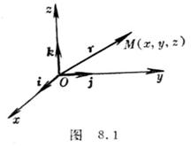 A vector whose starting point coincides with the origin O and ends at a point M
The quantity ( Fig. 8.1) is called the vector radius ( or radial ) of the point M , and is written as![]()
r , the origin is called the pole.Ifthe Cartesian coordinates of M are x , y , z ,
then there are
r ==( x , y , z )= x i + y j + z k![]()
where i , j , k are the positive units of the x - axis, y - axis, and z -axis, respectively
A vector, called a coordinate unit vector ( or basis vector ).
[Basic formula of vector]
|
name |
formula |
graphics |
|
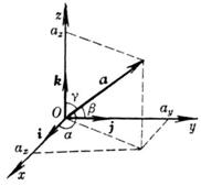
Coordinate representation of vector a coordinate unit vector i , j , k Coordinate representation of Coordinate representation of the zero vector the length(or modulus) of a The direction cosine of a (,, is the direction angle of a ) Vector ( both ends A , The coordinates of B are ( a x , a y , a z ), ( b x , b y , b z ) |
a = a x i + a y j + a z k =( a x , a y , a z ) i =(1,0,0) j =(0,1,0) k =(0,0,1) 0 = ( 0 , 0, 0 ) ( 0 has no direction ) + ( b z - a z ) k |
|
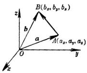
[Addition] If a = ( a x , a y , a z ) and b = ( b x , b y , b z ) , then
a + b =( a x + b x , a y + b y , a z + b z )
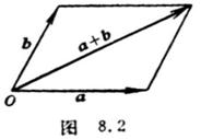
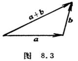
Move the starting point of the vector to the origin O , use a and b as sides to make a parallelogram, and the diagonal line drawn from the origin represents the sum vector a + b ( called the parallelogram rule, see Figure 8.2); End to end , the vector from the start point to the end point is the sum vector a + b ( called the triangle rule, see Figure 8.3).
The addition operation is governed by the following rules:
![]() ( commutative law )
( commutative law )
![]() ( associativity )
( associativity )
a + 0 = 0 + a = a , a +( - a )= 0
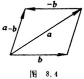
[Subtraction] If a = ( a x , a y , a z ) and b = ( b x , b y , b z ) , then
a - b =( a x - b x , a y - b y , a z - b z )
Add the negative vector of vector b to vector a to get vector a - b
( Figure 8.4).
The triangle inequality holds for any two vectors a and b :
| a + b | | a | + | b |![]()
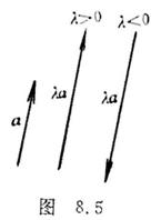
[Number multiplication] Multiplying a real number by a vector a is called number multiplication, denoted as a . When > 0, the modulus of a is stretched twice, and the direction remains unchanged; when < 0, the modulus of a is stretched | | times, and the direction is the same as a Conversely ( Figure 8.5) , if a = ( a x , a y , a z ) then ![]()
![]()
![]()
![]()
![]()
![]()
![]() a =( a x , a y , a z )
a =( a x , a y , a z )![]()
![]()
![]()
Let , be two real numbers, a and b are two vectors, then the multiplication operation is suitable for![]()
![]()
The following rules:
![]() (
( ![]() a ) = ( )
a ) = ( ) ![]()
![]() a
( associative law )
a
( associative law )
( ![]() + ) a = a + a ( distributive law )
+ ) a = a + a ( distributive law )![]()
![]()
![]()
![]() ( a + b ) = a + b ( distributive law )
( a + b ) = a + b ( distributive law )![]()
![]()
[Vector decomposition]
![]()
 1
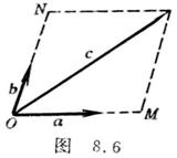
1 ![]() Let a , b , and c be three coplanar vectors, and b and c are non-collinear vectors, if they are moved to a common starting point O , two lines parallel to a and b are drawn from the end point C of the vector c .
Let a , b , and c be three coplanar vectors, and b and c are non-collinear vectors, if they are moved to a common starting point O , two lines parallel to a and b are drawn from the end point C of the vector c .
A straight line, each intersecting a , b ( or extension ) at M , N ( Fig. 8.6) , then
c =+= a + b![]()
![]()
![]()
![]()
This is called the decomposition of vector c to a , b .
 2
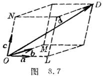
2 ![]() Let a , b , c be non-coplanar vectors, and d be any vector, let
Let a , b , c be non-coplanar vectors, and d be any vector, let
They move to a common starting point O , and three planes are drawn from the end point D of the vector d .
parallel to the ( b , c ) plane, ( c , a ) plane and ( a , b ) plane, and intersecting with a , b , c ( or extended lines ) at L , M , N respectively ( Fig. 8.7) , then
d =++= a + b +![]()
![]()
![]()
![]()
![]()
![]()
is called the decomposition of a , b , c of a vector d .
3 ![]() If two non-zero vectors a and b have a linear relationship
If two non-zero vectors a and b have a linear relationship
![]() a + b = 0
a + b = 0![]()
In the formula , if not all 0 , the two vectors are said to be collinear ( ie![]()
![]()
a // b ); vice versa.Call these two vectors a , b linearly correlated.
4 ![]() Let a and b be two non-zero vectors, if a + b = 0 , then there are = 0, = 0, then a and b are said to be linearly independent .
Let a and b be two non-zero vectors, if a + b = 0 , then there are = 0, = 0, then a and b are said to be linearly independent .![]()
![]()
![]()
![]()
5 ![]() If the three non-zero vectors a , b , c have a linear relationship a + b + = 0 , where , , are not all zero, then these three vectors are coplanar, and vice versa . At this time, we call a , b , c is linear correlation . If a , b , c are three non-zero vectors, and a + b + = 0 , then = = = 0, at this time , a , b , c are said to be linearly independent .
If the three non-zero vectors a , b , c have a linear relationship a + b + = 0 , where , , are not all zero, then these three vectors are coplanar, and vice versa . At this time, we call a , b , c is linear correlation . If a , b , c are three non-zero vectors, and a + b + = 0 , then = = = 0, at this time , a , b , c are said to be linearly independent .![]()
![]()
![]()
![]()
![]()
![]()
![]()
![]()
![]()
![]()
![]()
![]()
6 ![]() Four ( or more than four ) vectors a , b , c , d must have a linear relationship; that is, they must be linearly related . At this time, there must be four numbers that are not all 0, , , , and a + b + + d = 0 .
Four ( or more than four ) vectors a , b , c , d must have a linear relationship; that is, they must be linearly related . At this time, there must be four numbers that are not all 0, , , , and a + b + + d = 0 .![]()
![]()
![]()
![]()
![]()
![]()
![]()
![]()
[scalar product ( quantity product, dot product, inner product ) ] Let a = ( a x , a y ,
a z ) , b = ( b x , b y , b z ) , | a | = a , | b | = b , the angle between the two vectors of a and b is _ _ _ ![]()
![]() ). denoted as
). denoted as
 a · b = ab = ab cos(
![]() 0)
0)![]()
![]()
![]()
![]()
It can be seen as the length of vector a multiplied by the length of the projection of vector b on a ( Figure 8.8).
The scalar product operation is subject to the following rules:
a · b = b · a
(commutative law)
a · ( b + c )= a · b + a · c (distributive law)
( ![]() a ) · ( b )
a ) · ( b ) ![]() = a · b ( associative law of multiplication )
= a · b ( associative law of multiplication )![]()
![]()
a · a = a 2 =| a | 2 = a 2
If a and b are non-zero vectors and a · b = 0, then a b![]() ; vice versa .
; vice versa .
i · i = j · j = k · k =1, i · j = j · k = k · i = 0
a · b = a x b x + a y b y + a z b z (that is, the sum of the multiplication of the corresponding coordinates)
[Vector product ( cross product, outer product ) ] Let a = ( a x , a y , a z ) , b = ( b x , b y , b z ) , | a | = a , | b | = b , The angle between the two vectors of a and b is _ _ _ ![]() That is, the length is equal to the area of a parallelogram with sides a and b ( shaded part in Figure 8.9 )
That is, the length is equal to the area of a parallelogram with sides a and b ( shaded part in Figure 8.9 )
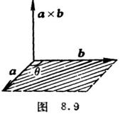 | a × b | = ab sin (
 ![]() 0 )
0 )![]()
![]()
![]()
![]()
Its direction is perpendicular to the two vectors a and b , and a , b , a × b constitute
Right-handed system ( Figure 8.9).
The vector product operation is subject to the following rules:
a × b =- b × a
(inverse commutative law)
( a + b ) × c = a × c + b × c
( distributive law, order cannot be exchanged )
( ![]() a ) × ( b )
a ) × ( b ) ![]() = ( a × b )
= ( a × b )![]()
![]()
[( ![]() + ) a ] × b = ( + )( a × b ) = ( a × b ) + ( a × b )
+ ) a ] × b = ( + )( a × b ) = ( a × b ) + ( a × b )![]()
![]()
![]()
![]()
![]()
a × a = 0
If a and b are non-zero vectors, the necessary and sufficient conditions for a and b to be collinear ( that is, a // b ) are:
a × b = 0
i × i = j × j = k × k = 0 , i × j = k , j × k = i , k × i = j
a × b ==( a y b z - a z
b y ) i +( a z b x - a x b z ) j + ( a x
b y - a y
b x ) k
[ Angle of two vectors ]
cos( a , b ) =![]()
sin( a , b ) =![]()
[ Lagrange identity ]
( a × b ) · ( c × d ) = ( a · c )( b · d ) - ( a · d )( b · c )
Special ( a × b ) 2 = a 2 b 2 - ( a b ) 2
i.e. ( a y
b x - a z b y ) 2 +( a z
b x - a x
b z ) 2 +( a x b y - a y b x ) 2
= ( a x 2 + a y 2 + a z 2 )( b x 2 + b y 2 + b z 2 ) - ( a x b x +a y b y +a z b z ) 2
[ Mixed product of three vectors ] Let a = ( a x , a y , a z ) , b = ( b x , b y , b z ) and c = ( c x , c y , c z ) be three vector , then their mixed product is defined as
( a bc ) = a · ( b × c ) = = a x ( b y c z - b z c y ) + a y ( b z c x - b x c z ) + a z ( b x c y - b y c x )
A mixed product has the properties :
1 a · ( b × c ) = ( a × b ) · c![]()
Note that in general the equation
( a · b ) · c = a · ( b · c )
( a × b ) × c = a × ( b × c )
not established .
2 ( ![]() a bc ) = ( bc a ) = ( c a b )= - ( a cb )= - ( b a c )= - ( cb a )
a bc ) = ( bc a ) = ( c a b )= - ( a cb )= - ( b a c )= - ( cb a )
That is, there is rotation:
a · ( b × c )= b · ( c × a )= c · ( a × b )= - a ( c × b )= - b ( a × c )= - c ( b × a )
3 A ![]() mixed product ( a bc ) is a number whose absolute value is equal to the volume of a parallelepiped with sides a , b , c .
mixed product ( a bc ) is a number whose absolute value is equal to the volume of a parallelepiped with sides a , b , c .
4 ![]() The necessary and sufficient conditions for the three vectors to be coplanar are: ( a bc ) = 0.
The necessary and sufficient conditions for the three vectors to be coplanar are: ( a bc ) = 0.
[ triple vector product ]
a × ( b × c ) = ( a · c ) b -( a · b ) c
( a × b ) × c = ( a · c ) b - ( b · c ) a
By using a , b , c rotation method, the other two similar formulas can also be derived .
[ Several formulas for multiple products ]
a ×( b × c )+ b ×( c × a )+ c ×( a × b ) = 0
( a × b ) · ( c × d ) = = ( a · c )( b · d ) - ( a · d )( b · c )![]()
( a × b ) × ( c × d ) = ( a bd ) c − ( a bc ) d = ( cd a ) b − ( cdb ) a
a ×[ b ×( c × d )]=( b · d )( a × c )-( b · c )( a × d )
( a × b b × c c × a ) = ( a bc ) 2
( a 1 a 2 a 3 )( b 1 b 2 b 3 ) =
( a × b c × d e × f ) = ( a bd )( cef ) − ( a bc )( def )
2. Vector analysis
1 . vector differentiation
[ Vector function ] For each value of the independent variable t ( scalar ) , there is a certain amount of change vector a ( a vector whose length and direction are determined ) and it corresponds to it, then the change ( vector ) amount a is called the vector of variable t . function, denoted
a = f ( t )
The vector function can also be expressed as
a = a x i + a y j + a z k
in the formula
a x = f x ( t ), a y = f y ( t ), a z = f z ( t )
are three scalar functions .
If the change vector is expressed as the radial vector form of point M
r = r ( t )
Then when t changes, the point M traces a curve in space, which is called the sagittal curve of the vector function . Its coordinates are given by three equations:
r = x i + y j + z k
x = x ( t ) , y = y ( t ) , z = z ( t )
[ Limit and Continuity of Vector Functions ] If for any given >0 , there is a number >0 such that when t - t 0 <![]()
![]()
![]()
![]()
![]()
![]() r ( t )− r 0 <
r ( t )− r 0 <![]()
![]()
is established, then r 0 is called the limit of the vector function r ( t ) when t t 0 , denoted as![]()
![]() = r 0
= r 0
If it exists, then![]()
![]() = i + j + k
= i + j + k![]()
![]()
![]()
If = r ( t 0 ), then the vector function r ( t ) is said to be continuous at t = t 0 . ![]()
[ Derivatives and Differentiation of Vector Functions ] If the limit
![]()
If it exists, it is called the derivative of the vector function a = f (t) , and denoted as . The derivative of the vector function a = f ( t ) is still a vector function, so its derivative can also be calculated, that is, the second derivative, denoted as , wait .![]()
![]()
d a = d t![]()
It is called the differentiation of the vector function a = f ( t ) .
[ Derivation formula of vector function ]
![]() = 0 ( c is a constant vector )
= 0 ( c is a constant vector )
![]() ( k a ) = k ( k is a constant )
( k a ) = k ( k is a constant )![]()
![]() ( a + b + c ) =
( a + b + c ) =![]()
![]() (
( ![]() a ) = a + ( is the scalar function of t )
a ) = a + ( is the scalar function of t )![]()
![]()
![]()
![]()
![]() ( a · b ) = · b + a · ( the order can be swapped )
( a · b ) = · b + a · ( the order can be swapped )![]()
![]()
![]() ( a × b ) = × b + a × ( orders cannot be swapped )
( a × b ) = × b + a × ( orders cannot be swapped )![]()
![]()
![]() ( a bc )=( bc )+(
( a bc )=( bc )+( ![]() a c )+( a b ) ( the order cannot be swapped )
a c )+( a b ) ( the order cannot be swapped )![]()
![]()
![]() a [( t )]=
a [( t )]=![]()
![]()
![]()
( ![]() is the scalar function of t , which is the derivation formula of the composite function )
is the scalar function of t , which is the derivation formula of the composite function )
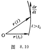
[ Formula for derivation of vector function in the form of vector radius ] Let
r = r ( t )= x ( t ) i + y ( t ) j + z ( t ) k
represents the end-of-vector curve of the vector function, then
1 = = i + j + k![]()
![]()
![]()
![]()
![]()
![]()
Represents the tangent vector of the sagittal curve ( Fig. 8.10) , pointing in the direction of increasing t , where = , = , =![]()
![]()
![]()
![]()
![]()
![]()
 2 = t
2 = t![]()
![]()
where s is the arc length of the sagittal curve, and t is the unit vector of the tangent .
3 ![]()
![]() = i + j + k
= i + j + k![]()
![]()
![]()
where = , = , =![]()
![]()
![]()
![]()
![]()
![]()
[ Taylor formula for vector functions ]
r ( t + t )= r ( t )+( t ) t +( t )( t ) 2 + ... + r ( n ) ( t )( t ) n + rn ( t ) n +1![]()
![]()
![]()
![]()
![]()
![]()
![]()
![]()
![]()
in the formula
r n = x ( n +1) ( t 1 ) i + y ( n +1) ( t 2 ) j + z ( n +1) ( t 3 ) k ( t < t 1 , t 2 , t 3 < t
+ t )![]()
r ( n ) ( t ) = x ( n ) ( t ) i + y ( n ) ( t ) j + z ( n ) ( t ) k
x ( n ) = , y ( n ) = , z ( n ) =![]()
![]()
![]()
[ Several common properties of vector functions ]
1 A fixed-length vector r ( t ) ( t ) , and vice versa . Thus the derivative of the unit vector t of the tangent is perpendicular to the original vector .![]()
![]()
![]()
2 ![]() Orientation vector r ( t )// ( t )
Orientation vector r ( t )// ( t ) ![]() and vice versa .
and vice versa .
3 A sufficient and necessary condition for ![]() a change vector r ( t ) to be parallel to a definite plane is: the mixed product
a change vector r ( t ) to be parallel to a definite plane is: the mixed product
( ) ![]()
![]()
![]() = 0
= 0
2 . vector integral
[ Indefinite integral ] Let a ( t ) and b ( t ) be vector functions, then the vector differential equation
![]() = a ( t )
= a ( t )
solution
![]() ( t )d t = b ( t ) + c ( where c is an arbitrary constant vector )
( t )d t = b ( t ) + c ( where c is an arbitrary constant vector )
is called the indefinite integral of the vector function a ( t ) .
[ Definite integral ]
Let a ( t ) and b ( t ) be vector functions, then
![]() a ( t )d t = b ( t 2 )− b ( t 1 )
a ( t )d t = b ( t 2 )− b ( t 1 )
It is called the definite integral of the vector function a ( t ) , and t1 and t2 are called the lower and upper limit, respectively .
[ plane area vector ] set
r = r ( t )= x ( t ) i + y ( t ) j + z ( t ) k
d r = i d x + j d y + k d z
but
S = r ×d r![]()
where L is the closed curve drawn by the vector end of r ( t ) , S is the area vector enclosed by L , and the origin is in the closed curve L.