§ 2
Field Theory Preliminary
1.
Basic Concepts of Field Theory and Gradient, Divergence and Curl
[ scalar field ] Each point M ( x , y , z ) in the space area D corresponds to a quantity value ( x , y , z ) , which constitutes a scalar field on this space area D , using the point M ( x,y , z ) is represented by the scalar function ( x , y , z ) . If the position of M is determined by the vector radius r , the scalar can be regarded as a function of the variable vector r = ( r ).![]()
![]()
![]()
![]()
![]()
For example, the temperature field u ( x , y , z ), the density field , and the electric potential field e ( x , y , z ) are all scalar fields .![]()
[ Vector field ] Each point M ( x , y , z ) in space area D corresponds to a vector value r ( x , y , z ) , which constitutes a vector field on this space area D , using point M ( x , y , z ) of the vector function r ( x , y , z ) is represented . If the position of M is determined by the vector radius r , the vector r can be regarded as the vector function r ( r of the variable vector r )) :
r ( r )= X ( x , y , z ) i + Y ( x , y , z ) j + Z ( x , y , z ) k
For example, the velocity field ( x , y , z ) , the electric field E ( x , y , z ) , the magnetic field H ( x , y , z ) are all vector fields . ![]()
As in the case of scalar fields, the concept of a vector field is essentially the same as that of a vector function . These terms ( scalar field, vector field ) are used to preserve their own origin and physical meaning .
[ gradient ]
grad ![]() = (
= ( ![]() , , ) = = i + j + k
, , ) = = i + j + k![]()
![]()
![]()
![]()
![]()
![]()
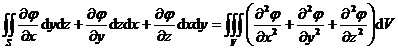
In the formula = i + j + k is called the Hamiltonian operator , also known as the Nepra operator. Grad is denoted as del in some books and periodicals .![]()
![]()
![]()
![]()
![]()
![]()
The direction of grad coincides with ![]() the normal direction N of the isometric plane = C passing through the points ( x , y , z ) , and points to the increasing side, which is the direction with the greatest rate of change of the function, and its length is equal to .
the normal direction N of the isometric plane = C passing through the points ( x , y , z ) , and points to the increasing side, which is the direction with the greatest rate of change of the function, and its length is equal to .![]()
![]()
![]()
![]()
Gradients have properties:
grad( ![]()
![]() + ) = grad + grad ( , is a constant )
+ ) = grad + grad ( , is a constant )![]()
![]()
![]()
![]()
![]()
![]()
![]()
grad( ) ![]()
![]() = grad + grad
= grad + grad![]()
![]()
![]()
![]()
grad F ( ) ![]() =
=![]()
[ Directional Derivative ]
![]() = l · grad
= l · grad ![]() = cos + cos + cos
= cos + cos + cos![]()
![]()
![]()
![]()
![]()
![]()
where l = (cos , cos , cos ) is ![]()
![]()
![]() the unit vector of direction l , , , which is the direction angle .
the unit vector of direction l , , , which is the direction angle .![]()
![]()
![]()
The directional derivative is the law of change in the direction l , which is equal to the projection of the gradient in the direction l .![]()
[ divergence ]
div r = + + = r = div ( X , Y , Z )![]()
![]()
![]()
![]()
where is the Hamiltonian .![]()
Divergence has the property:
div( ![]() a + b ) = div a + div b ( , is a constant )
a + b ) = div a + div b ( , is a constant )![]()
![]()
![]()
![]()
![]()
div( ![]() a ) = div a + a grad
a ) = div a + a grad![]()
![]()
div ( a × b ) = b rot a − a rot b _
[ curl ]
rot r = ( ) i![]() + ( ) j
+ ( ) j![]() + ( ) k
+ ( ) k![]() = × r =
= × r =![]()

where is Hamiltonian operator, curl is also called vorticity, rot r is denoted as curl r in some books and periodicals .![]()
Curl has the properties:
rot( ![]() a + b ) = rot a + rot b ( , is a constant )
a + b ) = rot a + rot b ( , is a constant )![]()
![]()
![]()
![]()
![]()
rot( ![]() a ) = rot a + a × grad
a ) = rot a + a × grad![]()
![]()
rot( a × b ) = ( b · ) a − ( a · ) b + (div b ) a − (div a ) b![]()
![]()
[ Gradient, divergence, curl mixed operation ] The operation grad acts on a scalar field to generate a vector field grad , the operation div acts on a vector field r to generate a scalar field div r , and the operation rot acts on a vector field r to generate a new vector field![]()
![]()
rot
r . The mixed operation formula of these three operations is as follows:
div rot r = 0
rot grad ![]() = 0
= 0
div grad ![]() = + + =
= + + =![]()
![]()
![]()
![]()
![]()
grad div r = ( r )![]()
![]()
rot rot r = × ( × r )![]()
![]()
div grad( + ) = div grad + div grad ( ![]()
![]()
![]()
![]()
![]()
![]()
![]()
![]() , is a constant )
, is a constant )![]()
div grad( )= div grad ![]()
![]()
![]()
![]() + div grad +2 grad · grad
+ div grad +2 grad · grad![]()
![]()
![]()
![]()
grad div r - rot rot r = r![]()
where is the Hamiltonian, and = = 2 is the Laplace operator . ![]()
![]()
![]()
![]()
![]()
[ Potential field ( conservation field )] If the vector field r ( x , y , z ) is the gradient of a scalar function ( x , y , z ) , that is![]()
r =grad![]() or X =, Y =, Z =
or X =, Y =, Z = ![]()
![]()
![]()
Then r is called the potential field, and the scalar function is called the potential function of r .![]()
The necessary and sufficient conditions for the vector field r to be a potential field are: rot r = 0, or
![]() = , = , =
= , = , =![]()
![]()
![]()
![]()
![]()
Potential function calculation formula
![]() ( x , y , z ) = ( x 0 , y 0 , z 0 ) + +
( x , y , z ) = ( x 0 , y 0 , z 0 ) + +![]()
![]()
![]()
+![]()
[ No scatter ( tubular field )] If the divergence of the vector field r is zero, that is, div r = 0 , then r is called a scatter-free field . At this time, there must be a scatter-free field T , so that r = rot T , for any point M has
T =![]()
![]()
where r is the distance from dV to M , and the integration is performed over the entire space .
[ Irrotational field ] If the curl of the vector field r is zero, that is, rot r = 0 , then r is called an irrotational field . The potential field is always an irrotational field, and there must be a scalar function , so that r = grad , and for any point M we have![]()
![]()
![]() =-
=-![]()
![]()
where r is the distance from d V to M , and the integration is performed over the entire space .
2.
Expressions of gradient, divergence and curl in different coordinate systems
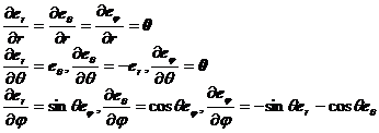
1 . unit vector transformation
![]() [ General formula ] Assume that x = f ( ), y = g ( ), z = h ( )
[ General formula ] Assume that x = f ( ), y = g ( ), z = h ( ) ![]()
![]()
![]() to continuously map a region of ( )
to continuously map a region of ( ) ![]() space to a region D of ( x , y , z ) space , and Assuming that f , g , h have continuous partial derivatives, because the correspondence is one-to-one, we have
space to a region D of ( x , y , z ) space , and Assuming that f , g , h have continuous partial derivatives, because the correspondence is one-to-one, we have
![]()
![]() = ( x , y , z ) ,
= ( x , y , z ) ,![]()
![]()
Assuming that there are also continuous partial derivatives, then we have![]()
or inverse transform
The unit vectors along the d x , dy , d z directions are denoted as i , j , k , and the unit vectors along the directions are denoted as![]()
![]()
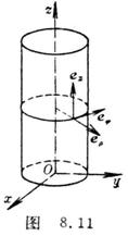
[ Unit vector of cylindrical coordinate system ] For cylindrical coordinate system ( Fig. 8.11)

![]()
The unit vector is
Their partial derivatives are
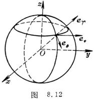
[ Unit vector of spherical coordinate system ] For spherical coordinate system ( Fig. 8.12)
![]()
The unit vector is
Their partial derivatives are
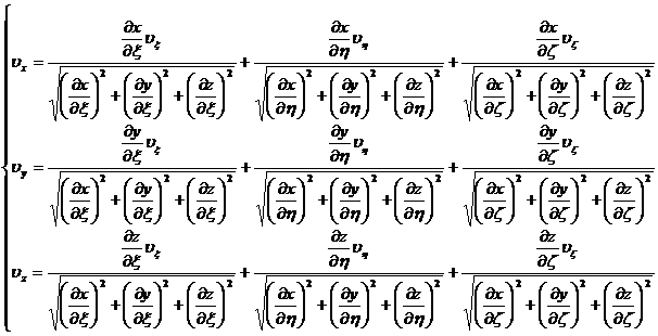
2 . Coordinate transformation of vectors
[ General formula ] A vector expressed by the ( x , y , z ) coordinate system can be expressed by the ( ) coordinate system :![]()
![]() = (
= ( ![]() , y , z ) = i + y j + z k =
, y , z ) = i + y j + z k =![]()
![]()
![]()
![]()
![]()
![]()
in the formula
[ Exchange of Cylindrical Coordinate System and Cartesian Coordinate System ] Transformation Formula from Cylindrical Coordinate System to Cartesian Coordinate System
Transformation formula from Cartesian coordinate system to cylindrical coordinate system
[ Exchange of spherical coordinate system and rectangular coordinate system ] Transformation formula from spherical coordinate system to rectangular coordinate system
Transformation formula from rectangular coordinate system to spherical coordinate system
3 . Expressions of various operators in different coordinate systems
Let U = U ( x , y , z ) be a scalar function and V = V ( x , y , z ) be a vector function .
[ Expressions of various operators in the cylindrical coordinate system ]
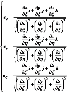
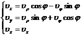
Hamiltonian = + + ![]()
![]()
![]()
![]()
Gradient grad U = U = + + ![]()
![]()
![]()
![]()
Divergence div V = · V = _ ![]()
![]()
Curl rot V = × V = + + _ ![]()
Laplacian U = div grad U = ![]()
![]()
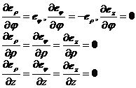
[ Expressions of various operators in spherical coordinates ]
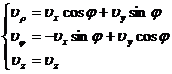
Hamiltonian = + + ![]()
![]()
![]()
![]()
Gradient grad U = U = + + ![]()
![]()
![]()
![]()
Divergence div V = · V = ![]()
![]()
Curl rot V = × V = _ ![]()
![]()
+![]()
![]()
+![]()
![]()
Laplacian U = div grad U ![]()
=![]()
3.
Curve integral, surface integral and volume derivative
[ Curve integral of a vector and its calculation formula ] The curvilinear integral of a vector field r ( r ) along a curve is defined as![]()
![]() r ( r )·d r = r ()· r i -1
r ( r )·d r = r ()· r i -1
![]()
![]()
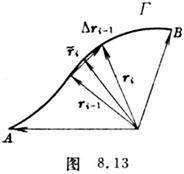 where ri -1 = ri - ri -1 , the right limit is independent of the choice of the curve
![]()
![]()
![]() From A to B ( Fig. 8.13)
From A to B ( Fig. 8.13)
If the vector function R ( r ) is continuous ( that is, its three components are
continuous function ), the curve is also continuous and has continuous rotation![]()
tangent , the curve integral
![]()
exist .
If R ( r ) is a force field, then P = equals to![]()
The work done by a force R when a particle moves along G.
The formula for calculating the vector curve integral is as follows:
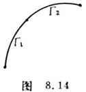
![]() =
=![]()
![]() =
= ![]() + ( Figure 8.14)
+ ( Figure 8.14)![]()
![]() = -
= -![]()
![]() =
= ![]() +
+![]()
![]() = k ( k
= k ( k![]() is a constant )
is a constant )
[ Circulation of the vector ] If G is a closed curve, then the curve integral along the curve G
![]() =
=![]()
It is called the circulation of the vector field R ( r ) along the closed curve G.
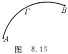 The circulation of the potential field along any closed curve is equal to zero . If R ( r ) is a potential field and its potential function is , then the curve integral
![]()
![]() =
= ![]() = ( B ) - ( A )
= ( B ) - ( A )![]()
![]()
It has nothing to do with the path connecting points A and B , but only depends on the path between points A and B.
position ( Figure 8.15).
[ Surface integral of a vector ] Let S be a surface, let N = denote the normal unit vector of a point on the surface S , V and d S = N d S denote the area vector element . Let ( r ) = ( x , y , z ) is a continuous scalar function defined on the surface S , R ( r )=( X ( x , y , z ), Y ( x , y , z ), Z![]()
![]()
![]() ( x ,
y , z )) is a continuous vector function defined on the surface S , the surface integral has the following three forms:
( x ,
y , z )) is a continuous vector function defined on the surface S , the surface integral has the following three forms:
1 Flux ( or flow ) of a scalar field![]()
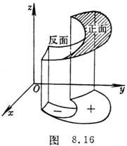
![]() d S = d y d zi
d S = d y d zi![]() + d z d x j + d x d y k _
+ d z d x j + d x d y k _![]()
![]()
where S yz , S zx , S xy represent the surface S in the Oyz plane, Ozx plane, respectively ,
Projection on the Oxy plane . The sign of S xy is specified as follows: when looking from the positive z axis
When looking to the side, what you see is the front of the surface S , consider S xy to be positive, if
If you see the opposite side of the surface, consider S xy to be negative ( Figure 8.16).
2 ![]() Scalar Flux of a Vector Field
Scalar Flux of a Vector Field
![]() R d S = X d y d z + Y d z d x + Z d x d y _
R d S = X d y d z + Y d z d x + Z d x d y _![]()
![]()
![]()
The meanings of S yz etc. in the formula are the same as 1 .![]()
3 ![]() Vector flux of a vector field
Vector flux of a vector field
![]() R ×d S =( Z j - Y k )d y d z +( X k - Z i )d z d x +( Y i - X j )d x d y
R ×d S =( Z j - Y k )d y d z +( X k - Z i )d z d x +( Y i - X j )d x d y![]()
![]()
![]()
The meanings of S yz etc. in the formula are the same as 1 .![]()
[ Volume Derivative of Vector ] If S is a closed surface enclosing volume V and contains point r , then the ratio of the surface integral ( d S , R d S , R × d S ) along the closed surface S to the volume V , when The limit when V tends to zero ( i.e. its diameter 0 ) is called the volume derivative ( or spatial derivative ) of the scalar field ( or vector field R ) at point r ).![]()
![]()
![]()
![]()
![]()
![]()
1 The volume derivative of a scalar field is its gradient:![]()
![]()
grad ![]() =
=
2 One of the volume derivatives of a ![]() vector field R is its divergence:
vector field R is its divergence:
div
R =
3 Another volume derivative of the ![]() vector field R is its curl:
vector field R is its curl:
rot
R = -
4.
Integral Theorem of Vectors
[ Gaussian formula ]
![]() R d V = R
R d V = R![]() · d S = R
· d S = R![]() · N d S
· N d S
which is
 where S is the boundary surface of the space region V , and N = is
![]()
normal unit vector at a point on S , R ( r )=( X ( x , y , z ), Y ( x , y , z ), Z ( x , y , z ))
There are continuous partial derivatives on V + S.
[ Stokes formula ]
![]() rot R · d S = rot R · N d S = R · d r
rot R · d S = rot R · N d S = R · d r![]()
![]()
which is
=
=![]()
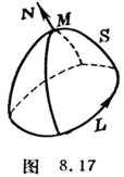
In the formula, S is one side of a certain surface, L is the closed boundary curve of the surface S ( the positive direction of L and N form a right-handed system ). Each point of S has a tangent surface, and its direction continuously depends on the points on the surface, and the boundary Each point on the curve L has a tangent ( Fig. 8.17). R ( r )=( X ( x ,
y , z ), Y ( x ,
y , z ), Z ( x ,
y , z )) at the surface of the All points are single-valued and have continuous partial derivatives at points close enough to S.
[ Green formula ]
![]() · dS = _
· dS = _![]()
![]() · dS = _
· dS = _![]()
In the formula, S is the boundary surface of the space region V , which is two scalar functions. It has continuous partial derivatives on S and second-order continuous partial derivatives on V. It is the Laplace operator, especially![]()
![]()
![]() · dS = _
· dS = _![]()
which is