info prev up next book cdrom email home

Newton-Cotes Formulas

The Newton-Cotes formulas are an extremely useful and straightforward family of Numerical Integration techniques.


To integrate a function $f(x)$ over some interval $[a,b]$, divide it into $n$ equal parts such that $f_n = f(x_n)$ and $h
\equiv (b-a)/n$. Then find Polynomials which approximate the tabulated function, and integrate them to approximate the Area under the curve. To find the fitting Polynomials, use Lagrange Interpolating Polynomials. The resulting formulas are called Newton-Cotes formulas, or Quadrature Formulas.


Newton-Cotes formulas may be ``closed'' if the interval $[x_1,x_n]$ is included in the fit, ``open'' if the points $[x_2,x_{n-1}]$ are used, or a variation of these two. If the formula uses $n$ points (closed or open), the Coefficients of terms sum to $n-1$.


If the function $f(x)$ is given explicitly instead of simply being tabulated at the values $x_i$, the best numerical method of integration is called Gaussian Quadrature. By picking the intervals at which to sample the function, this procedure produces more accurate approximations (but is significantly more complicated to implement).
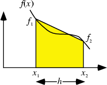

\begin{figure}\begin{center}\BoxedEPSF{TrapezoidalRule.epsf}\end{center}\end{figure}

The 2-point closed Newton-Cotes formula is called the Trapezoidal Rule because it approximates the area under a curve by a Trapezoid with horizontal base and sloped top (connecting the endpoints $x_1$ and $x_2$). If the first point is $x_1$, then the other endpoint will be located at

$\displaystyle x_2$ $\textstyle =$ $\displaystyle x_1+h,$ (1)

and the Lagrange Interpolating Polynomial through the points $(x_1,f_1)$ and $(x_2,f_2)$ is
$\displaystyle P_2(x)$ $\textstyle =$ $\displaystyle {x-x_2\over x_1-x_2} f_1+{x-x_1\over x_2-x_1}f_2$  
  $\textstyle =$ $\displaystyle {x-x_1-h\over -h} f_1+{x-x_1\over h} f_2$  
  $\textstyle =$ $\displaystyle {x\over h} (f_2-f_1)+\left({f_1+{x_1\over h}f_1-{x_1\over h} f_2}\right).$ (2)

Integrating over the interval (i.e., finding the area of the trapezoid) then gives


$\displaystyle \int_{x_1}^{x_2} f(x)\,dx$ $\textstyle =$ $\displaystyle \int_{x_1}^{x_1+h} P_2(x)\,dx$  
  $\textstyle =$ $\displaystyle {1\over 2h} (f_2-f_1) [x^2]_{x_1}^{x_2}+ \left({f_1+{x_1\over h}f_1-{x_1\over h} f_2}\right)[x]_{x_1}^{x_2}\hfill$  
  $\textstyle =$ $\displaystyle {1\over 2h} (f_2-f_1)(x_2+x_1)(x_2-x_1)+(x_2-x_1)\left({f_1+{x_1\over h}f_1-{x_1\over h} f_2}\right)\hfill$  
  $\textstyle =$ $\displaystyle {\textstyle{1\over 2}}(f_2-f_1)(2x_1+h)+f_1h+x_1(f_1-f_2)$  
  $\textstyle =$ $\displaystyle x_1(f_2-f_1)+{\textstyle{1\over 2}}h(f_2-f_1)+hf_1-x_1(f_2-f_1)$  
  $\textstyle =$ $\displaystyle {\textstyle{1\over 2}}h(f_1+f_2)-{\textstyle{1\over 2}}h^3 f''(\xi).$ (3)

This is the trapezoidal rule, with the final term giving the amount of error (which, since $x_1\leq\xi\leq x_2$, is no worse than the maximum value of $f''(\xi)$ in this range).


The 3-point rule is known as Simpson's Rule. The Abscissas are

$\displaystyle x_2$ $\textstyle =$ $\displaystyle x_1+h$ (4)
$\displaystyle x_3$ $\textstyle =$ $\displaystyle x_1+2h$ (5)

and the Lagrange Interpolating Polynomial is

$P_3(x)={(x-x_2)(x-x_3)\over (x_1-x_2)(x_1-x_3)} f_1+{(x-x_1)(x-x_3)\over (x_2-x_1)(x_2-x_3)}f_2+{(x-x_1)(x-x_2)\over (x_3-x_1)(x_3-x_2)} f_3$
$={x^2-x(x_2+x_3)+x_2x_3\over h(2h)} f_1+{x^2-x(x_1+x_3)+x_1x_3\over h(-h)}f_2+{x^2-x(x_1+x_2)+x_1x_2\over 2h(h)}f_3$
$={1\over h^2} \{x^2({\textstyle{1\over 2}}f_1-f_2-{\textstyle{1\over 2}}f_3)+x[-{\textstyle{1\over 2}}(2x_1+3h)f_1+(2x_1+2h)f_2-{\textstyle{1\over 2}}(2x_1+h)]$
$+[{\textstyle{1\over 2}}(x_1+h)(x_1+2h)f_1-x_1(x_1+2h)f_2+{\textstyle{1\over 2}}x_1(x_1+h)f_3]\}.\quad$ (6)
Integrating and simplifying gives


\begin{displaymath}
\int_{x_1}^{x_3} f(x)\,dx = \int_{x_1}^{x_1+2h} P_3(x)\,dx =...
... 3}} h(f_1+4f_2+f_3)-{\textstyle{1\over 90}} h^5 f^{(4)}(\xi).
\end{displaymath} (7)


The 4-point closed rule is Simpson's 3/8 Rule,

\begin{displaymath}
\int_{x_1}^{x_4} f(x)\,dx = {\textstyle{3\over 8}} h (f_1+3f_2+3f_3+f_4) -{\textstyle{3\over 80}} h^5 f^{(4)}(\xi).
\end{displaymath} (8)

The 5-point closed rule is Bode's Rule,


\begin{displaymath}
\int_{x_1}^{x_5} f(x)\,dx = {\textstyle{2\over 45}} h (7f_1+32f_2+12f_3+32f_4+7f_5)-{\textstyle{8\over 945}} h^7 f^{(6)}(\xi)
\end{displaymath} (9)

(Abramowitz and Stegun 1972, p. 886). Higher order rules include the 6-point


\begin{displaymath}
\int_{x_1}^{x_6} f(x)\,dx = {\textstyle{5\over 288}} h (19f_...
...4+75f_5+19f_6) -{\textstyle{275\over 12096}} h^7 f^{(6)}(\xi),
\end{displaymath} (10)

7-point
$\int_{x_1}^{x_7} f(x)\,dx = {\textstyle{1\over 140}} h (41f_1+216f_2+27f_3+272f_4$
$+27f_5+216f_6+41f_7)-{\textstyle{9\over 1400}} h^9 f^{(8)}(\xi),\quad$ (11)
8-point
$\int_{x_1}^{x_8} f(x)\,dx = {\textstyle{7\over 17280}} h (751f_1+3577f_2+1323f_2+2989f_3$
$+2989f_5+1323f_6+3577f_7+751f_8)-{\textstyle{8183\over 518400}} h^9 f^{(8)}(\xi),$

(12)
9-point

$\int_{x_1}^{x_9} f(x)\,dx = {\textstyle{4\over 14175}} h (989f_1+5888f_2-928f_3+10496f_4-4540f_5+10496f_6-928f_7$
$ +5888f_8+989f_9)-{\textstyle{2368\over 467775}} h^{11} f^{(10)}(\xi),\quad$ (13)
10-point
$\int_{x_1}^{x_{10}} f(x)\,dx = {\textstyle{9\over 89600}} h [2857(f_1+f_{10})$
$ +15741(f_2+f_9)+1080(f_3+f_8+19344(f_4+f_7)$
$ +5788(f_5+f_6)]-{\textstyle{173\over 14620}} h^{11} f^{(10)}(\xi),\quad$ (14)
and 11-point
$\int_{x_1}^{x_{11}} f(x)\,dx = {\textstyle{5\over 299376}} h [16067(f_1+f_{11})$
$+106300(f_2+f_{10})-48525(f_3+f_9)+272400(f_4+f_8)$
$-260550(f_5+f_7)+427368f_6]-{\textstyle{1346350\over 326918592}} h^{13} f^{(12)}(\xi)$

(15)
rules.


Closed ``extended'' rules use multiple copies of lower order closed rules to build up higher order rules. By appropriately tailoring this process, rules with particularly nice properties can be constructed. For $n$ tabulated points, using the Trapezoidal Rule $(n-1)$ times and adding the results gives
$\int_{x_1}^{x_n} f(x)\,dx = \left({\int_{x_1}^{x_2}+\int_{x_2}^{x_3}+\ldots+\int_{x_{n-1}}^{x_n}}\right)f(x)\,dx$
$ ={\textstyle{1\over 2}}h[(f_1+f_2)+(f_2+f_3)+\ldots+(f_{n-2}+f_{n-1})$
$+(f_{n-1}+f_n)]= h({\textstyle{1\over 2}}f_1+f_2+f_3+\ldots+f_{n-2}+f_{n-1}+{\textstyle{1\over 2}}f_n)$
$-{\textstyle{1\over 12}} nh^3f''(\xi).\quad$ (16)
Using a series of refinements on the extended Trapezoidal Rule gives the method known as Romberg Integration. A 3-point extended rule for Odd $n$ is

$\int^{x_n}_{x_1} f(x)\,dx = h[({\textstyle{1\over 3}} f_1+{\textstyle{4\over 3}...
...{\textstyle{1\over 3}}f_3+{\textstyle{4\over 3}}f_4+{\textstyle{1\over 3}} f_5)$
$+\ldots+({\textstyle{1\over 3}} f_{n-4} +{\textstyle{4\over 3}} f_{n-3}+{\texts...
...{1\over 3}} f_{n-2}+ {\textstyle{4\over 3}}f_{n-1}+{\textstyle{1\over 3}} f_n)]$
$={\textstyle{1\over 3}} h (f_1+4f_2+2f_3+4f_4+2f_5+\ldots+4f_{n-1}+f_n) - {n-1\over 2} {\textstyle{1\over 90}} h^5f^{(4)}(\xi).$ (17)
Applying Simpson's 3/8 Rule, then Simpson's Rule (3-point) twice, and adding gives

$\left[{\int_{x_1}^{x_4}+\int_{x_4}^{x_6}+\int_{x_6}^{x_8}}\right]f(x)\,dx$
$ = h[({\textstyle{3\over 8}} f_1+{\textstyle{9\over 8}}f_2+{\textstyle{9\over 8...
...{\textstyle{1\over 3}}f_6+{\textstyle{4\over 3}}f_7+{\textstyle{1\over 3}}f_8)]$
$ = h[{\textstyle{3\over 8}}f_1+{\textstyle{9\over 8}}f_2+{\textstyle{9\over 8}}...
...\textstyle{1\over 3}})f_6 +{\textstyle{4\over 3}}f_7+{\textstyle{1\over 3}}f_8]$
$ = h({\textstyle{3\over 8}}f_1+{\textstyle{9\over 8}}f_2+{\textstyle{9\over 8}}...
...tstyle{2\over 3}}f_6+{\textstyle{4\over 3}}f_7+{\textstyle{1\over 3}}f_8).\quad$ (18)
Taking the next Simpson's 3/8 step then gives

\begin{displaymath}
\int_{x_8}^{x_{11}} f(x)\,dx = h({\textstyle{3\over 8}}f_8+{...
..._9+{\textstyle{9\over 8}}f_{10}+{\textstyle{3\over 8}}f_{11}).
\end{displaymath} (19)

Combining with the previous result gives
$\int_{x_1}^{x_{11}} f(x)\,dx = h[{\textstyle{3\over 8}}f_1+{\textstyle{9\over 8...
...{\textstyle{9\over 8}}f_3+{\textstyle{17\over 24}}f_4+{\textstyle{4\over 3}}f_5$
$ +{\textstyle{2\over 3}}f_6+{\textstyle{4\over 3}}f_7+({\textstyle{1\over 3}}+{...
...tstyle{9\over 8}}f_9+{\textstyle{9\over 8}}f_{10}+{\textstyle{3\over 8}}f_{11}]$
$ = h({\textstyle{3\over 8}}f_1+{\textstyle{9\over 8}}f_2+{\textstyle{9\over 8}}...
...4+{\textstyle{4\over 3}}f_5+{\textstyle{2\over 3}}f_6+{\textstyle{4\over 3}}f_7$
$ +{\textstyle{17\over 24}}f_8+{\textstyle{9\over 8}}f_9+{\textstyle{9\over 8}}f_{10}+{\textstyle{3\over 8}}f_{11}),\quad$ (20)
where terms up to $f_{10}$ have now been completely determined. Continuing gives
$h({\textstyle{3\over 8}}f_1+{\textstyle{9\over 8}}f_2+{\textstyle{9\over 8}}f_3...
...tyle{17\over 24}}f_4+{\textstyle{4\over 3}}f_5+{\textstyle{2\over 3}}f_6+\ldots$
$\mathop{+}{\textstyle{2\over 3}}f_{n-5} +{\textstyle{4\over 3}}f_{n-4}+{\textst...
...ver 8}}f_{n-2}+{\textstyle{9\over 8}}f_{n-1}+{\textstyle{3\over 8}}f_{n}).\quad$ (21)
Now average with the 3-point result
\begin{displaymath}
h ({\textstyle{1\over 3}}f_1+{\textstyle{4\over 3}}f_2+{\tex...
...}}f_5+{\textstyle{4\over 3}}f_{n-1}+{\textstyle{1\over 3}}f_n)
\end{displaymath} (22)

to obtain
$h[{\textstyle{17\over 48}} f_1+{\textstyle{59\over 48}}f_2+{\textstyle{43\over 48}}f_4+{\textstyle{49\over 48}}f_4+(f_5+f_6+\ldots+f_{n-5}+f_{n-4})$
$\mathop{+}{\textstyle{49\over 48}}f_{n-3}+{\textstyle{43\over 38}}f_{n-2} +{\te...
...yle{59\over 48}}f_{n-1}+{\textstyle{17\over 48}}f_n]+{\mathcal O}(n^{-4}).\quad$ (23)
Note that all the middle terms now have unity Coefficients. Similarly, combining a 4-point with the (2+4)-point rule gives


\begin{displaymath}
h({\textstyle{5\over 12}}f_1+{\textstyle{13\over 12}}f_2+f_3...
...er 12}} f_{n-1}+{\textstyle{5\over 12}})+{\mathcal O}(n^{-3}).
\end{displaymath} (24)


Other Newton-Cotes rules occasionally encountered include Durand's Rule


\begin{displaymath}
\int_{x_1}^{x_n} f(x)\,dx = h({\textstyle{2\over 5}}f_1+{\te...
...-2}+{\textstyle{11\over 10}}f_{n-1}+{\textstyle{2\over 5}}f_n)
\end{displaymath} (25)

(Beyer 1987), Hardy's Rule

$\int_{x_0-3h}^{x_0+3h} f(x)\,dx = {\textstyle{1\over 100}}h(28f_{-3}+162f_{-2}+22f_0+162f_2+28f_3)$
$+{\textstyle{9\over 1400}}h^7 [2f^{(4)}(\xi_2)-h^2f^{(8)}(\xi_1)],\quad$ (26)
and Weddle's Rule


\begin{displaymath}
\int_{x_1}^{x_{6n}} f(x)\,dx = {\textstyle{3\over 10}} h(f_1+5f_2+f_3+6f_4+5f_5+f_6+\ldots+5f_{6n-1}+f_{6n})
\end{displaymath} (27)

(Beyer 1987).


The open Newton-Cotes rules use points outside the integration interval, yielding the 1-point

\begin{displaymath}
\int_{x_0}^{x_2} f(x)\,dx= 2hf_1,
\end{displaymath} (28)

2-point
$\int_{x_0}^{x_3} f(x)\,dx = \int_{x_1-h}^{x_1+2h} P_2(x)\,dx$
$= {1\over 2h} (f_2-f_1)[x^2]^{x_1+2h}_{x_1-h}+\left({f_1+{x_1\over h} f_1-{x_1\over h} f_2}\right)[x]^{x_1+2h}_{x_1-h} $
$={\textstyle{3\over 2}} h (f_1+f_2)+{\textstyle{1\over 4}}h^3 f''(\xi),\quad$ (29)
3-point
\begin{displaymath}
\int_{x_0}^{x_4} f(x)\,dx = {\textstyle{4\over 3}} h(2f_1-f_2+2f_3)+{\textstyle{28\over 90}} h^5 f^{(4)}(\xi),
\end{displaymath} (30)

4-point
\begin{displaymath}
\int_{x_0}^{x_5} f(x)\,dx = {\textstyle{5\over 24}} h (11f_1+f_2+f_3+11f_4) +{\textstyle{95\over 144}} h^5 f^{(4)}(\xi),
\end{displaymath} (31)

5-point


\begin{displaymath}
\int_{x_0}^{x_6} f(x)\,dx = {\textstyle{6\over 20}} h (11f_1...
...6f_3-14f_4+11f_5) -{\textstyle{41\over 140}} h^7 f^{(6)}(\xi),
\end{displaymath} (32)

6-point
$\int_{x_0}^{x_7} f(x)\,dx = {\textstyle{7\over 1440}} h (611f_1-453f_2+562f_3+562f_4$
$ -453f_5+611f_6)-{\textstyle{5257\over 8640}} h^7 f^{(6)}(\xi),\quad$ (33)
and 7-point
$\int_{x_0}^{x_8} f(x)\,dx = {\textstyle{8\over 945}} h (460f_1-954f_2+2196f_3-2459f_4$
$ +2196f_5-954f_6+460f_7) -{\textstyle{3956\over 14175}} h^9 f^{(8)}(\xi)\quad$ (34)
rules.


A 2-point open extended formula is
$\int_{x_1}^{x_n} f(x)\,dx= h[({\textstyle{1\over 2}}f_1+f_2+\ldots+f_{n-1}+{\textstyle{1\over 2}}f_n)$
$ +{\textstyle{1\over 24}}(-f_0+f_2+f_{n-1}-f_{n+1})]+ {11(n+1)\over 720} h^5f^{(4)}(\xi).$

(35)


Single interval extrapolative rules estimate the integral in an interval based on the points around it. An example of such a rule is

\begin{displaymath}
hf_1+{\mathcal O}(h^2f')
\end{displaymath} (36)


\begin{displaymath}
{\textstyle{1\over 2}}h(3f_1-f_2)+{\mathcal O}(h^3f'')
\end{displaymath} (37)


\begin{displaymath}
{\textstyle{1\over 12}} h(23f_1-16f_2+5f_3)+{\mathcal O}(h^4f^{(3)})
\end{displaymath} (38)


\begin{displaymath}
{\textstyle{1\over 24}} h(55f_1-59f_2+37f_3-9f_4)+{\mathcal O}(h^5f^{(4)}).
\end{displaymath} (39)

See also Bode's Rule, Difference Equation, Durand's Rule, Finite Difference, Gaussian Quadrature, Hardy's Rule, Lagrange Interpolating Polynomial, Numerical Integration, Simpson's Rule, Simpson's 3/8 Rule, Trapezoidal Rule, Weddle's Rule


References

Abramowitz, M. and Stegun, C. A. (Eds.). ``Integration.'' §25.4 in Handbook of Mathematical Functions with Formulas, Graphs, and Mathematical Tables, 9th printing. New York: Dover, pp. 885-887, 1972.

Beyer, W. H. (Ed.) CRC Standard Mathematical Tables, 28th ed. Boca Raton, FL: CRC Press, p. 127, 1987.

Hildebrand, F. B. Introduction to Numerical Analysis. New York: McGraw-Hill, pp. 160-161, 1956.

Press, W. H.; Flannery, B. P.; Teukolsky, S. A.; and Vetterling, W. T. ``Classical Formulas for Equally Spaced Abscissas.'' §4.1 in Numerical Recipes in FORTRAN: The Art of Scientific Computing, 2nd ed. Cambridge, England: Cambridge University Press, pp. 124-130, 1992.


info prev up next book cdrom email home

© 1996-9 Eric W. Weisstein
1999-05-25