A Tensor, also called a Riemannian Metric, which is symmetric and Positive Definite. Very roughly, the metric tensor  is a function which tells how to compute the distance between
any two points in a given Space. Its components can be viewed as multiplication factors which must be placed in
front of the differential displacements
is a function which tells how to compute the distance between
any two points in a given Space. Its components can be viewed as multiplication factors which must be placed in
front of the differential displacements  in a generalized Pythagorean Theorem
 |
(1) |
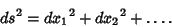
In Euclidean Space,
 where
where  is the Kronecker Delta (which is 0 for
  and
1 for
and
1 for  ), reproducing the usual form of the Pythagorean Theorem
 |
(2) |
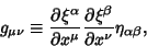
The metric tensor is defined abstractly as an Inner Product of every Tangent Space of a Manifold such
that the Inner Product is a symmetric, nondegenerate, bilinear form on a Vector Space. This means that it
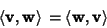
takes two Vectors
 as arguments and produces a Real Number
 such that
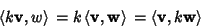 |
(3) |
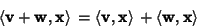 |
(4) |
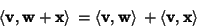 |
(5) |
 |
(6) |
 |
(7) |
with equality Iff  .
.
In coordinate Notation (with respect to the basis),
 |
(8) |
 |
(9) |
 |
(10) |
where
 is the Minkowski Metric. This can also be written
 |
(11) |
where
 |
(14) |
gives
 |
(15) |
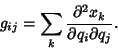
The metric is Positive Definite, so a metric's Discriminant is Positive. For a metric in 2-space,
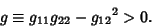 |
(16) |
The Orthogonality of Contravariant and Covariant metrics stipulated by
 |
(17) |
for  , ...,
  gives linear equations relating the
  quantities
and
quantities
and  . Therefore, if metrics are known, the others can be determined.
In 2-space,
If  is symmetric, then
In Euclidean Space (and all other symmetric Spaces),
 |
(23) |
so
 |
(24) |
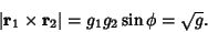
The Angle  between two parametric curves is given by
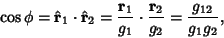 |
(25) |
so
 |
(26) |
and
 |
(27) |
The Line Element can be written
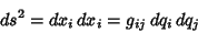 |
(28) |
where Einstein Summation has been used. But
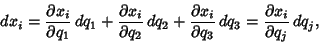 |
(29) |
so
 |
(30) |
For Orthogonal coordinate systems,  for , and the Line Element becomes (for 3-space)
where
 are called the Scale Factors.
See also Curvilinear Coordinates, Discriminant (Metric), Lichnerowicz Conditions, Line Element,
Metric, Metric Equivalence Problem, Minkowski Space, Scale Factor, Space
© 1996-9 Eric W. Weisstein
1999-05-26